FishEye Knowldge Graph: Identify Temporal Patterns of individual entities and between entities
VAST Chaellenge 2023: Mini-Challenge 2
(First Published: Jun 04, 2023)
1.Overview 🎣
1.1 Setting the Scene
The country of Oceanus has sought FishEye International’s help in identifying companies possibly engaged in illegal, unreported, and unregulated (IUU) fishing. As part of the collaboration, FishEye’s analysts received import/export data for Oceanus’ marine and fishing industries. However, Oceanus has informed FishEye that the data is incomplete. To facilitate their analysis, FishEye transformed the trade data into a knowledge graph. Using this knowledge graph, it hopes to understand business relationships, including finding links that will help stop IUU fishing and protect marine species that are affected by it.
1.2 Our Task
In response to Question 1 of VAST Chaellenge 2023: Mini-Challenge 2, our tasks are to:
Use visual analytics to identify temporal patterns for individual entities and between entities in the knowledge graph FishEye created from trade records, and
Categorize the types of business relationship patterns we can identify.
2.Set Up 🐠
2.1 Load the relevant packages into the R environment
We use the pacman::p_load() function to load the required R packages into our working environment. The loaded packages are:
igraph : provides functions for creating, analyzing, and visualizing graphs
ggraph: creates visualizations of graphs using the grammar of graphics approach
visNetwork : creates interactive network visualizations
graphlayouts : provides layout algorithms for graph visualization
jsonlite : for working with JSON (JavaScript Object Notation) data
plotly : for creating interactive web-based graphs
patchwork : for combining multiple plots into a single layout
knitr: for dynamic report generation
kableExtra : provides additional customization options for tables created with the knitr package,
DT : creates interactive tables using the DataTables JavaScript library
treemap : for creating treemaps
2.2 Import and Extract the data
The given data is a directed knowledge graph provided in json format. It contains 2 sets of information _ Nodes and Edges attributes .
- We first imported data as assign it to a variable mc2.
- Next. we extracted the nodes information from mc2 data frame
The nodes data frame contains the following attributes:
id -- Name of the company that originated (or received) the shipment
shpcountry -- Country the company most often associated with when shipping
rcvcountry -- Country the company most often associated with when receiving
- Then we extracted the edges info from mc2 data frame
The edges data frame contains the following attributes:
arrivaldate -- Date the shipment arrived at port in YYYY-MM-DD format.
hscode -- Harmonized System code for the shipment. Can be joined with the hscodes table to get additional details.
valueofgoods_omu -- Customs-declared value of the total shipment, in Oceanus Monetary Units (OMU)
volumeteu -- The volume of the shipment in ‘Twenty-foot equivalent units’, roughly how many 20-foot standard containers would be required. (Actual number of containers may have been different as there are 20ft and 40ft standard containers and tankers that do not use containers)
weightkg -- The weight of the shipment in kilograms (if known)
Since these working files are huge, we stored the mc2 nodes and edges data frames in rds format for ease of subsequent retrieval. This code need only be executed once. Thereafter we reloaded the mc2_nodes and edges data frames for data wrangling.
2.3 Data Preparation
2.3.1 Edge Data Frame
Inspect the data frame
We gott some summary statistics to understand the edge data.
    source             target           arrivaldate            hscode
 Length:5464378     Length:5464378     Min.   :2028-01-01   Length:5464378
 Class :character   Class :character   1st Qu.:2029-09-11   Class :character
 Mode  :character   Mode  :character   Median :2031-04-30   Mode  :character
                                       Mean   :2031-05-31
                                       3rd Qu.:2033-02-25
                                       Max.   :2034-12-30

 valueofgoods_omu           volumeteu                 weightkg
 Min.   :    1100.00000   Min.   :   0.000000000   Min.   :        0.000000
 1st Qu.:  148130.00000   1st Qu.:   0.000000000   1st Qu.:     3060.000000
 Median :  504485.00000   Median :   0.000000000   Median :    10300.000000
 Mean   : 1665142.29537   Mean   :   1.471786376   Mean   :    37265.707968
 3rd Qu.: 1202560.00000   3rd Qu.:   0.000000000   3rd Qu.:    19730.000000
 Max.   :44744530.00000   Max.   :1215.000000000   Max.   :495492485.000000
 NA's   :5464097          NA's   :520933
 valueofgoodsusd
 Min.   :           0.0000
 1st Qu.:       26815.0000
 Median :       72040.0000
 Mean   :      865446.5412
 3rd Qu.:      158030.0000
 Max.   :225833730200.0000
 NA's   :3017844
The following are noted:
There are 7 years of transactions, ranging from 1-Jan-2028 to 30-Dec-2034
Valueofgood_omu, volumeteu and valueofgoodusd attributes contain a lot of ’NA’s. These attributes are not useful for our analysis.
Check for the presence of duplicate records
We were unsure of the reasons behind the duplicate records and did not discount the possibility that they could be genuine. On balance, we found it unlikely that duplicate records exist for every day, with same weight and among the same pair of entities. Hence, we used the distinct() function on the edge data to only retain only unique edge records for our analysis.
2.3.2 Identify edge records that relate to the fishing industry
We referred to the HS Nomenclature 2022 available at World Customs Organisation (WCO)’s website, and the HSN Code List that is provided by Connect2India on their website. Based on these sources, we identified the following HS codes that correspond to different categories of fishery and seafood items.
| HS Code | Description |
|---|---|
| 3-digit code | |
| - 301 | Live fish |
| - 302 | Fish, fresh or chilled, whole |
| - 303 | Fish, frozen, whole |
| - 304 | Fish fillets, fish meat, mince except liver, roe |
| - 305 | Fish,cured, smoked, fish meal for human consumption |
| - 306 | Crustaceans |
| - 307 | Molluscs |
| - 308 | Fish and crustaceans, molluscs and other aquatic |
Next, we imported the list of relevant HS codes and the descriptions into our work environment and used the information to extract records related to the fishery products
Show the code
# Import the relevant HS codes
hscode_fish <- read_csv('data/lookup_hscode.csv', show_col_types = FALSE ) %>%
  mutate(hscode = as.character(hscode))

# Filter by 3-digit and 4-digit HS codes for fishery products
mc2_edges_fish <- mc2_edges_unique %>%
  filter(hscode %in% hscode_fish$hscode) %>%
  filter(substr(hscode,start = 1,stop=3) %in% c('301','302','303','304','305','306','307','308')
           )
We did a frequency count by hscode and list the top 20 transacted HS codes to gain a better understanding of the number of transactions and the quantities that were involved.
Show the code
freq_count_fish <- mc2_edges_fish %>%
  group_by(hscode) %>%
  summarise(count = n(),
            sum_weight = sum(weightkg)) %>%
  inner_join(hscode_fish,select(hscode,short_desc),by = 'hscode')

top_10 <- freq_count_fish %>%
  arrange(desc(count)) %>%
  head(10) %>%
  mutate(short_desc = as.character(short_desc))

rest <- freq_count_fish %>%
  filter(!(hscode %in% top_10$hscode)) %>%
  summarise(count = sum(count),
            sum_weight = sum(sum_weight)) %>%
  mutate(hscode = "others",
         short_desc = "Other fishery products")

final_df <- bind_rows(top_10, rest)

ggplot(final_df, aes(x = reorder(short_desc, -count), y = count)) +
  geom_bar(stat = "identity", fill = "skyblue", alpha = 0.8) +
  labs(x = "HS Code Short Description", y = "Count",
       title = "Top 10 Fishery Products Transacted between 2028 And 2034",
       caption = "Transactions for the other 148 6-digit HS Codes are categorised under 'Other fishery products'") +
  theme_minimal() +
  coord_flip() +
  theme(axis.text.x = element_text(hjust = 1),
        plot.title = element_text(hjust = 0, margin = margin(t = 20, r = 0, b = 10, l = 0)))
2.4.Community Detection
The filtered edge records contain 8.9k entities with 538.2k links. A network of this size was too complex for us to conduct a meaningful analysis visually. As nodes within the same community tend to have more interactions among themselves than with nodes in other communities, we partitioned them into communities and then select one community to study. This made it easier to analyze the chosen community’s transformation over time and interpret the network’s organization,
2.4.1 Identify the community of interest for our subsequent analysis
- To begin, we identified all unique pairs of transacting entities from the 538.2k links by removing self-links (i.e. source = target) and filtering away transactions that occurred fewer than 3 times over the 7 years (i.e < 1 transaction a year on average).
Show the code
mc2_edges_aggregated2 <- mc2_edges_fish %>%
  mutate(weeknumber = isoweek(arrivaldate),
         year = year(arrivaldate)) %>%
  group_by(source,target) %>%
  summarise(weight=n(),weight_sum = sum(weightkg)) %>%
  filter(source != target) %>%
  # filter away edge pairs that only had 3 transactions over the 7 years
  filter(weight >3) %>%
ungroup()- Next, we prepared the nodes data using the unique pairs of transacting entities.
Show the code
mc2_nodes_aggregated2 <- mc2_nodes %>%
  filter(id  %in% c(mc2_edges_aggregated2$source, mc2_edges_aggregated2$target)) %>%
  # Duplicate the id column as this name will be replaced once we convert to when we apply tbl_graph()
  mutate(label = id) %>%
  arrange(label) %>%
  mutate(row_id = row_number()) %>%
distinct() - Thereafter, we prepared the graph object, and apply the Walktrap Algorithm for community detection.
Show the code
# Create graph object
# Note that we are using an directed graph for this analysis and we can't use the popular louvain algo as the latter only applies to undirected graphs in r.
mc2_graph2 <- tbl_graph(nodes=mc2_nodes_aggregated2,edges = mc2_edges_aggregated2, directed = T)


set.seed(1234)

# Convert ggraph to igraph object
igraph_obj <- as.igraph(mc2_graph2)

# Detection algo. This algo accepts directed graph and is fast
community <- cluster_walktrap(igraph_obj, weights= E(igraph_obj)$weight)
membership <- community$membership
Results ==> 2.4k communities were detected with only the top 28 communities having more than 10 entities.
Show the code
# Count the occurrences of each membership value
membership_counts <- table(membership)

# Sort the table by membership counts in decreasing order
sorted_membership <- sort(membership_counts, decreasing = TRUE)

# Create a data frame from the sorted membership data
membership_data <- data.frame(Community_Id = names(sorted_membership[1:30]),
                              Count = as.numeric(sorted_membership[1:30]))

# Create a DT table from the membership data frame
membership_table <- datatable(membership_data,
                              options = list(pageLength = 5
                                            ),
                              caption = "Table 1: Top 30 Communities Detected and their membership size") %>%
  formatStyle(1,
                target = 'row',
                backgroundColor = styleEqual(c(14), c('#c7e9c0')))

# Display the DT table
membership_table
We chose the community with id=14 for our analysis, which consists of 164 nodes/entities. This community is the second largest one in our dataset and it offers a good trade-off between complexity and clarity. We wanted to avoid a graph that is too dense or too sparse for our study.
Show the code
# Extract community id 14 from the main graph
subgraph_3 <-as.directed(induced_subgraph(igraph_obj, community$membership==14))

# Extract nodes of the community
subgraph_nodes_info <- subgraph_3 %>%
  as_tbl_graph() %>%
  activate(nodes) %>%
  select(-id) %>%
  mutate(id = row_number()) %>%
  as_tibble()

# Extract edges of the community
subgraph_edge_info <- subgraph_3 %>%
  as_tbl_graph() %>%
  activate(edges) %>%
  inner_join(subgraph_nodes_info,select(id,label), by=c('from'='id')) %>%
  rename(source = label) %>%
    inner_join(subgraph_nodes_info,select(id,label), by=c('to'='id')) %>%
  rename(target = label) %>%
  select(source,target) %>%
  as_tibble()
2.4.2 Extract the nodes and edge information of the selected community
We then extracted the edges records for the unique pairs of transacting entities in community id = 14 from the m2_edges_fish (this is data frame that we extracted in Section 2.3.2. after extracting the desired the HS Codes) as we needed to retrieve their yearly transactions. At the same time, we re-labeled and replaced the values in the id column as the entity names within the column could be overwritten when we generate the graph object.
Show the code
# Extract the edge info from original graph
subgraph_edges2 <- mc2_edges_fish %>%
  mutate(weeknumber = isoweek(arrivaldate),
         year = year(arrivaldate)) %>%
  filter(source  %in% subgraph_edge_info$source, target  %in% subgraph_edge_info$target) %>%
  group_by(source,target,year,hscode) %>%
  summarise(weight=n(),
            sum_weight = sum(weightkg)) %>%
  ungroup() %>%
  inner_join(select(hscode_fish, hscode, short_desc), by = "hscode")

# Re-label and replace the values in the id column
subgraph_nodes2 <- mc2_nodes %>%
  filter(id  %in% c(subgraph_edges2$source, subgraph_edges2$target)) %>%
  # Duplicate the id column as this name will be replaced once we convert to when we apply tbl_graph()
  mutate(label = id) %>%
  arrange(label) %>%
  mutate(row_id = row_number()) %>%
  distinct()

# Replace with NA values in shpcountry and rcvcountry to prevent downstream issue
subgraph_nodes2 <- replace(subgraph_nodes2, is.na(subgraph_nodes2), 'unknown')
Finally, we generated the graph object.
At this point, we had the following objects for Community id 14:
subgraph_edge2
subgraph_nodes2
subgraph_obj: A
tbl_graph()object created using the nodes and edges information
2.4.3 Exploratory Data Analysis of the Community
- Year-on-Year trend of the number and quantity of fishery products transactions
Show the code
# Y-oY plot by weight
weight_yoy <- subgraph_edges2 %>%
  group_by(year) %>%
  summarise(sum_weight2=round(sum(sum_weight)/1000,0)) %>%
  ungroup()

ggplot(weight_yoy, aes(x = year, y = sum_weight2)) +
  geom_line(color = "#1f77b4", size = 1.5) +
  geom_text(aes(label = sum_weight2), vjust = -0.5) +
  scale_y_continuous(limits = c(0000, max(weight_yoy$sum_weight2) * 1.1)) +
  theme_minimal() +
  labs(x = "Year", y = "Total Weight\n(in tonnes)",
       title = 'Total Weight by Year') +
  theme(axis.title.y = element_text(angle = 0, vjust = 0.5, hjust=1))
Show the code
# Y-oY plot by count
count_yoy <- subgraph_edges2 %>%
  group_by(year) %>%
  summarise(count=sum(weight)) %>%
  ungroup()

ggplot(count_yoy, aes(x = year, y = count)) +
  geom_line(color = "#aec7e8", size = 1.5) +
  geom_text(aes(label = count), vjust = -0.5) +
  scale_y_continuous(limits = c(0, max(count_yoy$count) * 1.1)) +
  theme_minimal() +
  labs(x = "Year", y = "No. of Transactions",
       title = 'Transactions by Year') +
  theme(axis.title.y = element_text(angle = 0, vjust = 0.5, hjust=1))
There is a general uptrend in the number and quantity of fishery products transacted from Year 2028 to Year 2034
Noticeable surge in trade in Year 2033.
- Compute Centrality Measures for the Nodes
Show the code
subgraph_obj <- subgraph_obj %>%
  activate(nodes) %>%
  mutate(
          in_deg_centrality = round(centrality_degree(weights = weight, mode = "in", loops = FALSE),3),
          out_deg_centrality = round(centrality_degree(weights = weight, mode = "out", loops = FALSE),3),
          out_deg_closeness = round(centrality_closeness(weights=weight,mode='out',normalized = TRUE),3),
          in_deg_closeness = round(centrality_closeness(weights=weight,mode='in',normalized = TRUE),3),
          between_centrality = round(centrality_betweenness(weights = weight, directed = T),3)
          ) %>%
  mutate(in_deg_norm = round(ifelse(in_deg_centrality == 0, 0, (in_deg_centrality - min(in_deg_centrality)) / (max(in_deg_centrality) - min(in_deg_centrality))),3),
      out_deg_norm = round(ifelse(out_deg_centrality == 0, 0, ((out_deg_centrality - min(out_deg_centrality)) / (max(out_deg_centrality) - min(out_deg_centrality)))),3)
    )

# Create a tibble for display
nodes_stats <- subgraph_obj %>%
  activate(nodes) %>%
  as_tibble() %>%
  select(id,shpcountry,rcvcountry,in_deg_norm,out_deg_norm,between_centrality)

# Display the centrality measures for the nodes

datatable(nodes_stats, class = "compact", options = list(pageLength = 8),
              caption = "Table 2: Centrality Measures of Entities in Community",
rownames = FALSE)- Plot the static graph for the community
Show the code
set.seed(123)

g2_graph <- subgraph_obj %>%
  ggraph(layout = 'nicely') +
  geom_edge_link(aes(width=weight),
                 alpha=0.8) +
  scale_edge_width(range = c(0.05, 0.2)) +
  geom_node_point(aes(color=in_deg_norm, size = out_deg_norm, alpha=0.3)) +
  theme_graph() +
    labs(title = "Network Graph of Community Id 14 from Year 2028 to 2034") +
  theme(legend.position = "bottom")

g2_graph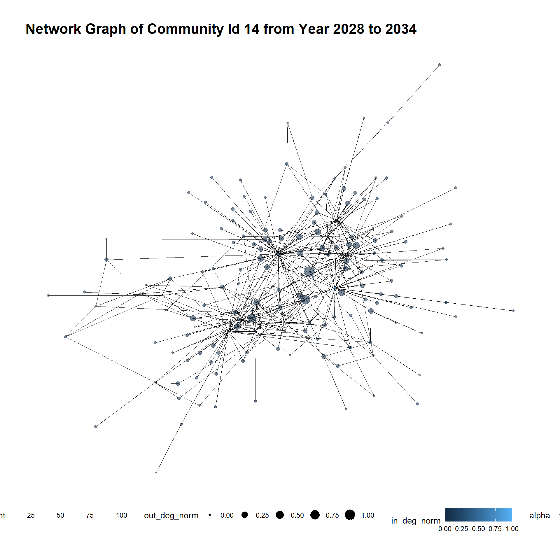
3.Identify temporal patterns for individual entities and between entities 🚢
In this section, we took a closer look at the transformation of Community Id 14 from Year 2028 to 2034 to understand how entities in the industry interacted over the 7 years. Before we begin, it’s crucial that we understand the visual cues that are used to appreciate the graphs
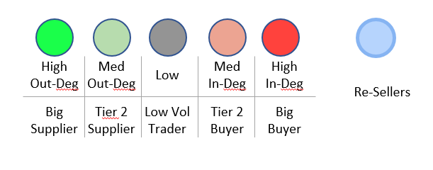
3.1 Undetstand the Visual Cues
| Visual Cue | Sample Image | What it means |
|---|---|---|
| Edges | ||
| - Arrow head | Refers to the direction in which shipment was made, A sends goods to B. | |
| - Edge width | 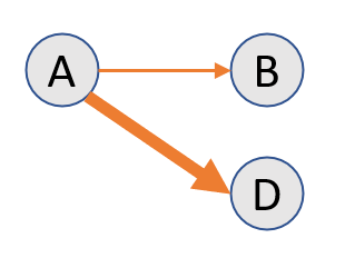 |
Thicker edge means there were more transactions between A and D than between A and B. |
| - Edge color | 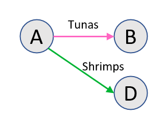 |
Different colored edges mean different seafood products (based on HS Code) were transacted between A and B, and A and D. |
| Nodes | ||
| - Color | 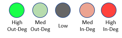 |
Entities that supply seafood do not usually re-sell them. Hence, most nodes were either a supplier or buyer. Bright green refers to suppliers with higher out-degrees and most would sell more fishery products by weight. At the other spectrum is the bright red nodes which relates bigger buyer with higher in-degrees. Again, most buyers (not all) would purchase more fishery products by weight. |
| - Label |  |
The label in the node is a reference for the entity involved. Only more active nodes (based on in-degree and out-degree centrality) are labelled. |
| - Edge Color |  |
A node with a pink ring indicates it is a re-seller, and possibly a transshipping entity. |
For each year, we created 3 functions to:
Plot the network graph
Compute the number of nodes and links involved
Treemaps which encode the number of transaction (size) and quantities involved (by color intensity) for In-degree and Out-degree nodes
Show the code
# Function to create network based on a given year and plot title
# Centrality measures for nodes are computed based on the year's network. Hence, these measures are not constant year on year

create_graph <- function(data, range, title) {

  set.seed(123)

  g <- data %>%
    #as_tbl_graph() %>%
    activate(edges) %>%
    filter(year %in% range) %>%
    activate(nodes) %>%
    mutate(
        in_deg_centrality = round(centrality_degree(weights = weight, mode = "in", loops = FALSE),3),
        out_deg_centrality = round(centrality_degree(weights = weight, mode = "out", loops = FALSE),3),
        out_deg_closeness = round(centrality_closeness(weights=weight,mode='out',normalized = TRUE),3),
        in_deg_closeness = round(centrality_closeness(weights=weight,mode='in',normalized = TRUE),3),
        between_centrality = round(centrality_betweenness(weights = weight, directed = T),3)
        ) %>%
    mutate(
      in_deg_norm = ifelse(in_deg_centrality == 0, 0, (in_deg_centrality - min(in_deg_centrality)) / (max(in_deg_centrality) - min(in_deg_centrality)) + 1),
      out_deg_norm = ifelse(out_deg_centrality == 0, 0, (1 - (out_deg_centrality - min(out_deg_centrality)) / (max(out_deg_centrality) - min(out_deg_centrality))))
    ) %>%
    mutate(combined_in_out_deg = in_deg_norm + out_deg_norm,
           bet_ind = ifelse(between_centrality >0, 1,0)) %>%
    mutate(row_id = ifelse((combined_in_out_deg>=1.2) | (combined_in_out_deg <=0.8),row_id,""))

  Isolated <- which(degree(g) == 0)
  g <- delete.vertices(g, Isolated)

  g %>%
    as_tbl_graph() %>%
    ggraph(layout = 'nicely') +
    geom_edge_link(aes(), alpha = 0.5) +
    geom_edge_fan(
      aes(color = short_desc),
      arrow = arrow(length = unit(2, 'mm')),
      end_cap = circle(3.3, 'mm'),
      start_cap = circle(3, 'mm')
    ) +
    geom_node_circle(aes(fill = combined_in_out_deg,r = 0.3, colour = bet_ind),alpha=0.8) +
    scale_fill_gradient2(low = "#20E620", mid = "#666666", high = "#E00000", midpoint = 1) +
    scale_color_gradient(low = "#666666", high = "pink")+
    geom_node_text(aes(label = row_id, size=0.5), colour = "black") +
    theme_graph() +
    theme(legend.position = "none") +
    labs(title = title) +
      coord_fixed()
}
Show the code
# Function to compute the number of nodes and links

cal_node_edges <- function(data, range) {
  # Convert tbl_graph to igraph object

  g <- data %>%
    #as_tbl_graph() %>%
    activate(edges) %>%
    filter(year %in% range)

  Isolated <- which(degree(g) == 0)
  igraph_obj <- delete.vertices(g, Isolated)

  # Convert tbl_graph object to igraph
  #igraph_obj = as.igraph(g)

  # Compute the number of nodes and edges
  num_nodes <- vcount(igraph_obj)
  num_edges <- ecount(igraph_obj)

  # Print the results
  df <- data.frame(Num_of_Nodes = num_nodes, Num_of_Edges = num_edges)

  print(df)
}
Show the code
# Create a function to create treemaps for in and out degree
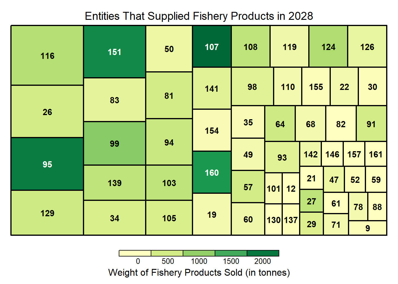
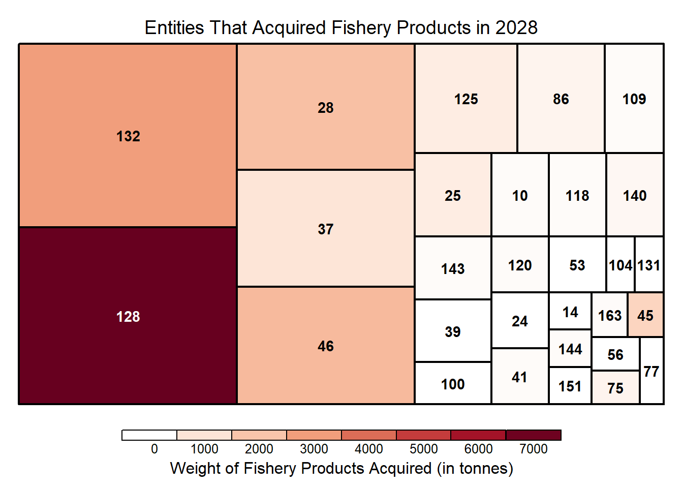
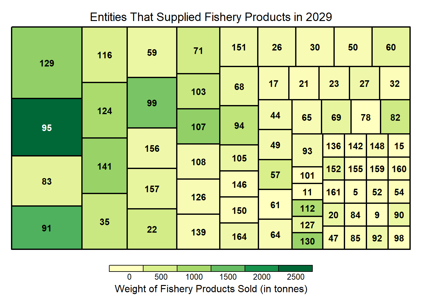
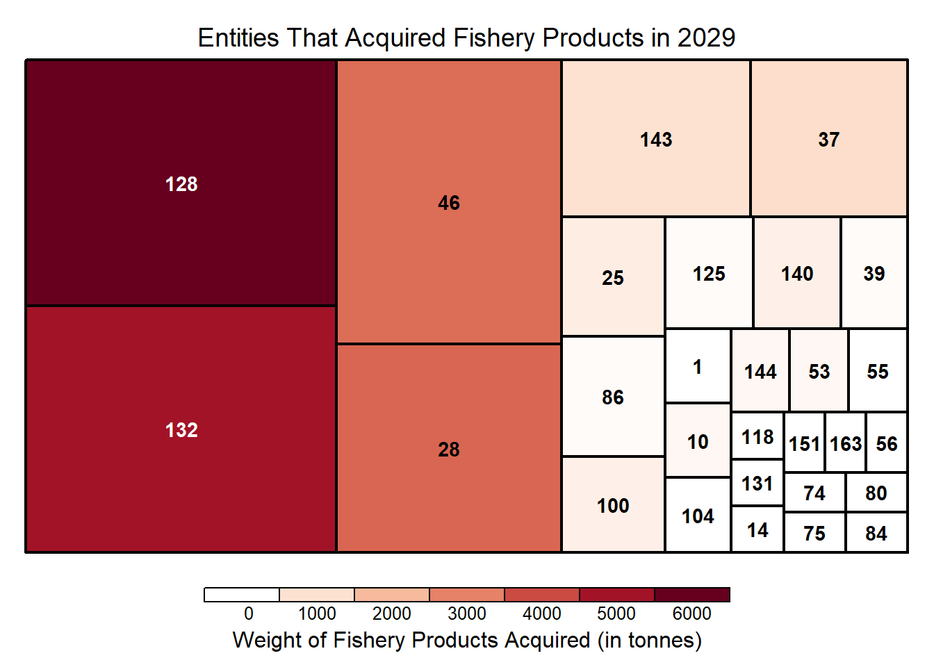
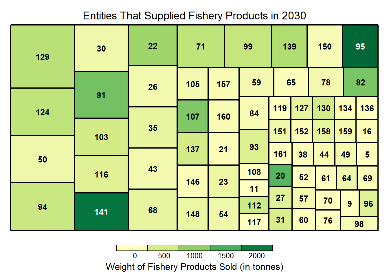
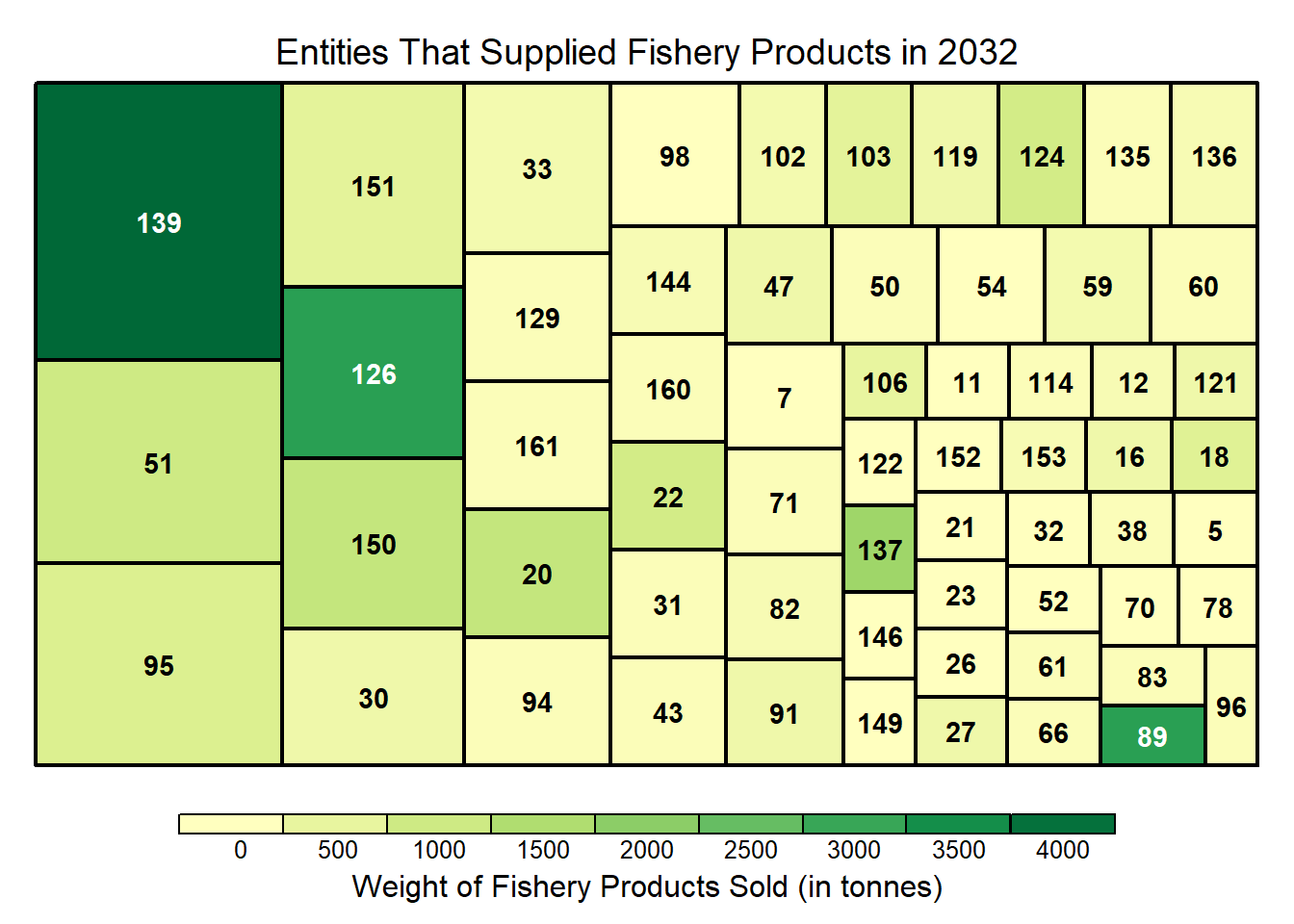
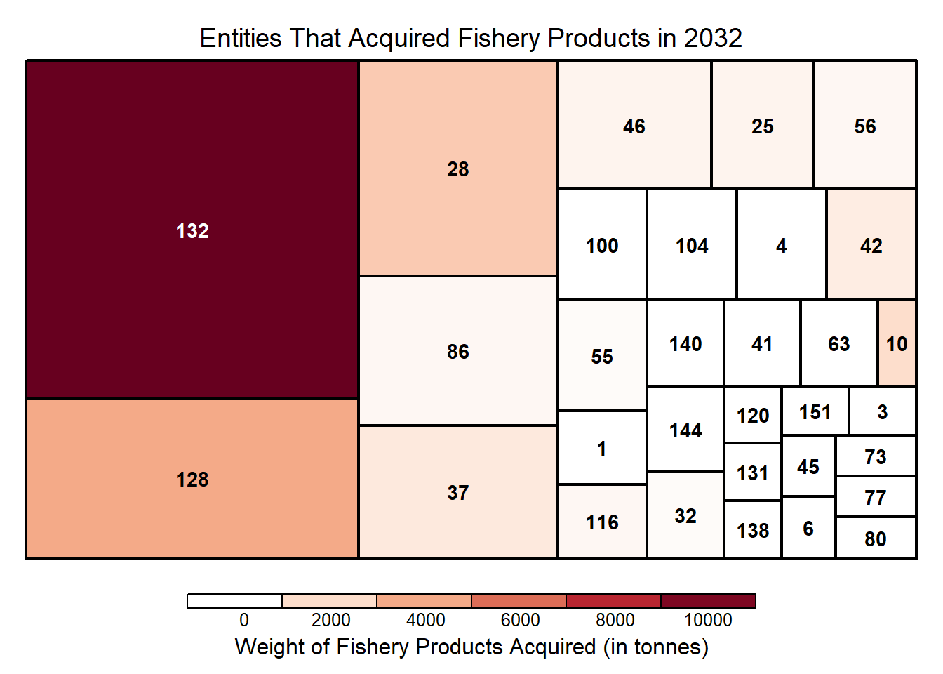
treemaps <- function(data, range) {
# Prepare the data
pivot_table <- data %>%
activate(edges)%>%
as.tibble() %>%
filter(year %in% range) %>%
group_by(from,to) %>%
summarise(count = n(),
sum_weight=sum(sum_weight)/1000) %>%
arrange(desc(sum_weight)) %>%
ungroup()
# Plot map for the suppliers
Suppliers <- treemap(pivot_table,
index=c("from"),
vSize="count",
vColor="sum_weight",
type = "value",
title= paste("Entities That Supplied Fishery Products in",range),
title.legend = "Weight of Fishery Products Sold (in tonnes)"
)
# Plot map for the buyers
Buyers <- treemap(pivot_table,
index=c("to"),
vSize="count",
vColor="sum_weight",
type = "value",
palette = "-RdGy",
title=paste("Entities That Acquired Fishery Products in",range),
title.legend = "Weight of Fishery Products Acquired (in tonnes)"
)
}3.2 Temporal Analysis of Individuals and between entities
Show the code
Show the code
Show the code
Show the code
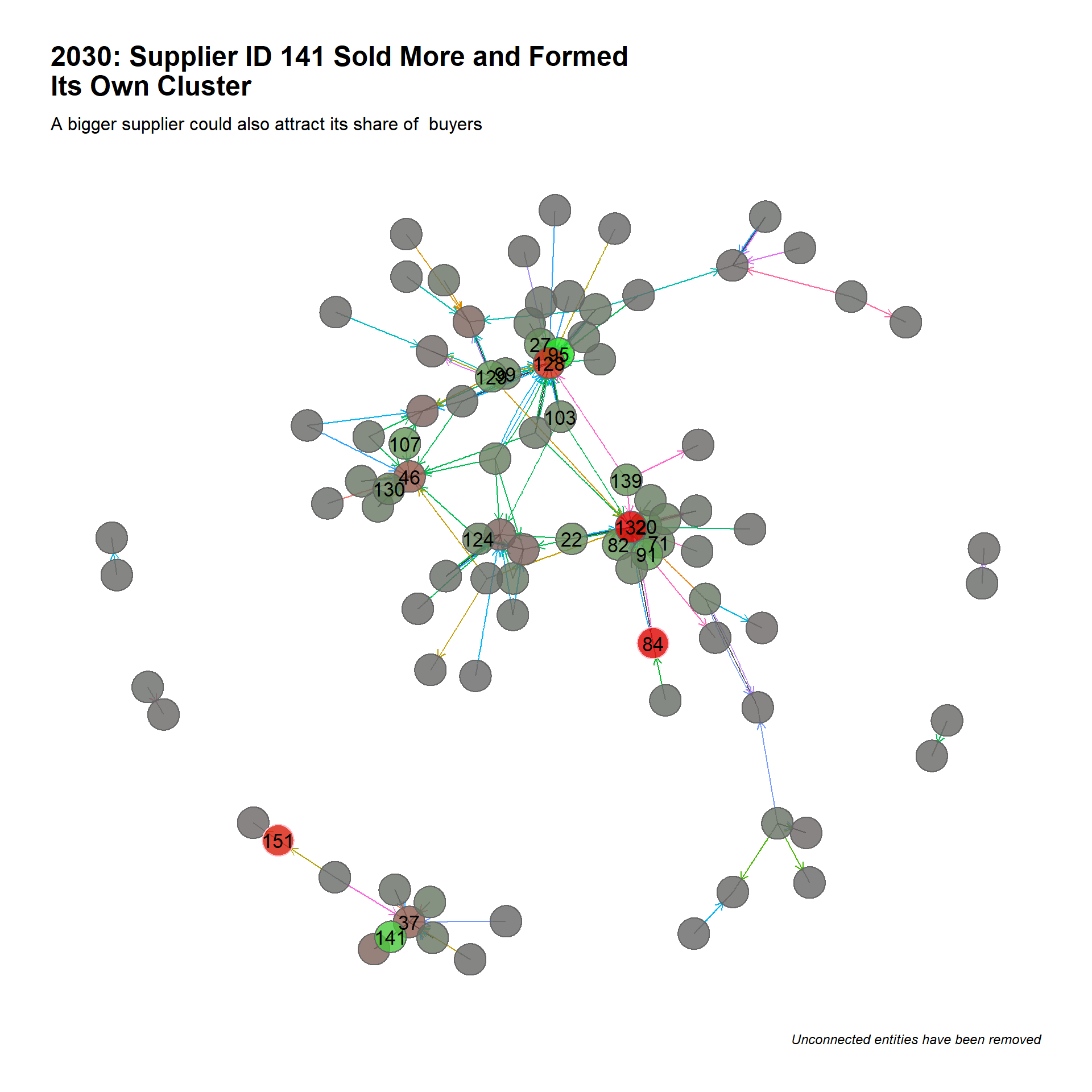
range <- c(2031)

create_graph(data,range,"2031: Supplier ID 139 Sold Much More Than Before\nwhile Supplier ID 141 Scaled Down its Business") +
  labs(subtitle="The increase in ID 139's supplies correlates with the increase in ID 132's purchase\nRe-seller ID 119 joined the network",
       caption = "Unconnected entities have been removed " )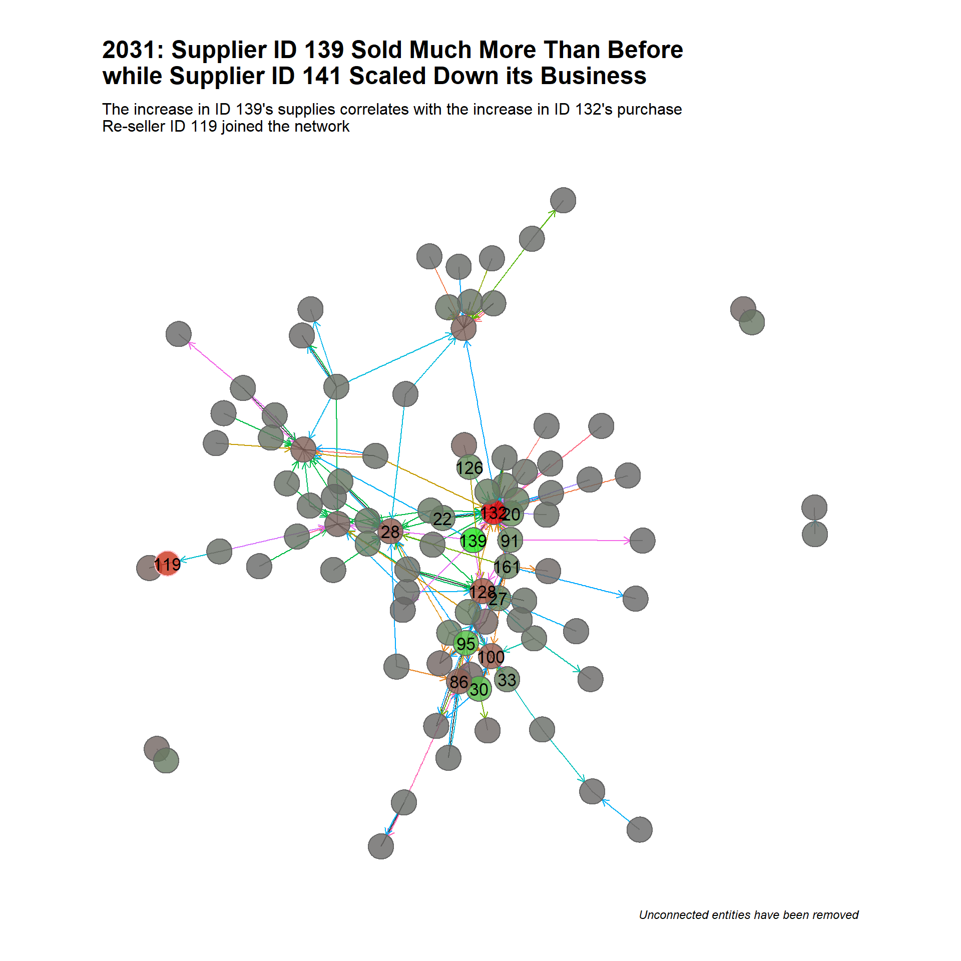
Show the code
range <- c(2032)
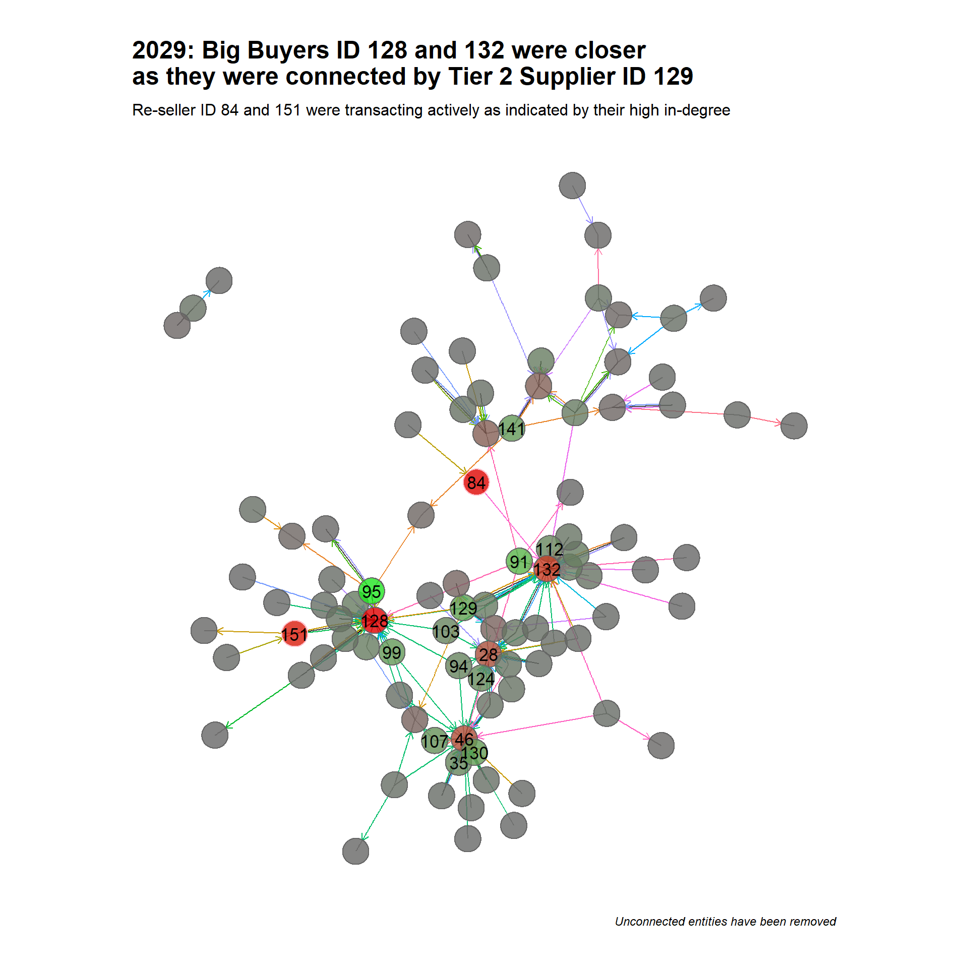
create_graph(data,range,"2032: Supplier ID 139 and Buyer ID 132\nDoniminated and Took Centre-stage in the Network") +
labs(subtitle="Bigger Supplier ID 95 which had around since 2028 left the network\nRe-seller ID 84 disappeared and new re-sellers ID 32 and 144 joined",
caption = "Unconnected entities have been removed " )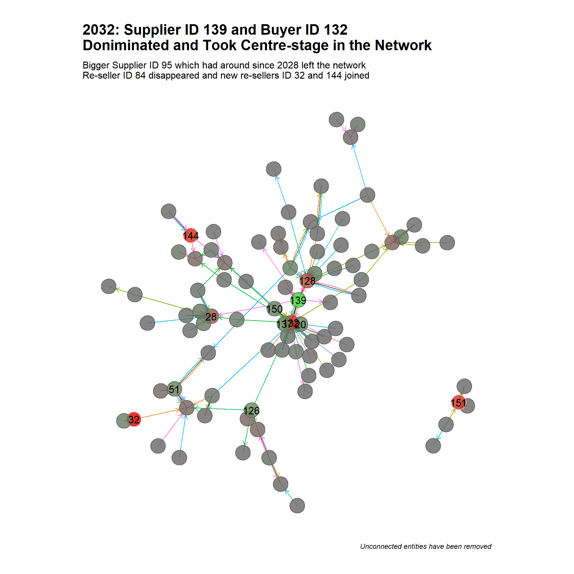
Show the code
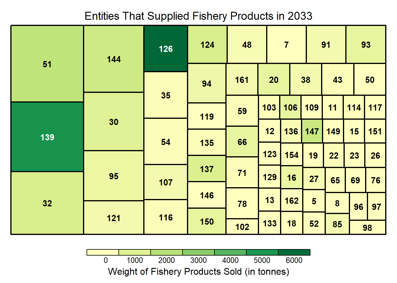
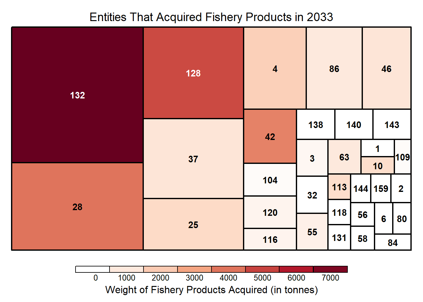
range <- c(2033)

create_graph(data,range,"2033: Resellers ID 32 and 144 Moved to the Centre\nof the Network Trading Actively with Various Entities")+
  labs(subtitle="In contrast to what we observed in 2028, we have a big supplier (ID 139) surrounded\nby a few smaller buyers",
       caption = "Unconnected entities have been removed " )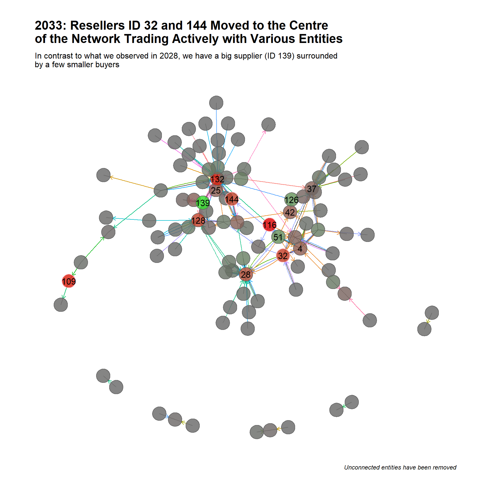
Show the code
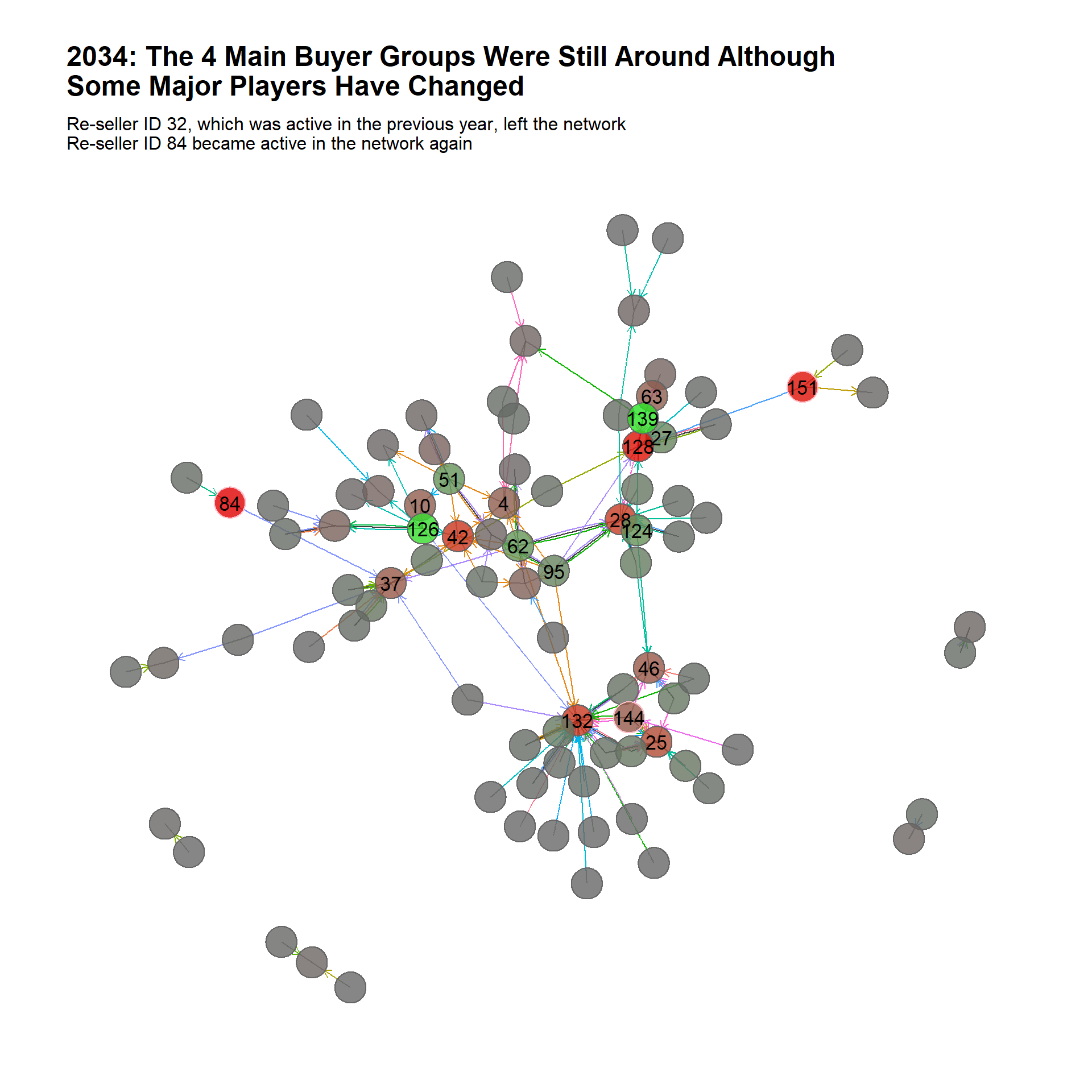
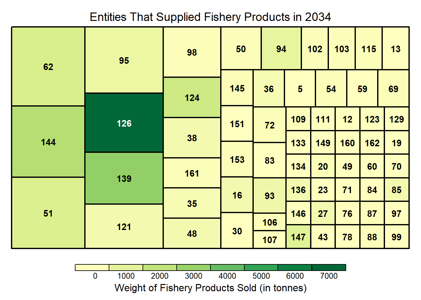
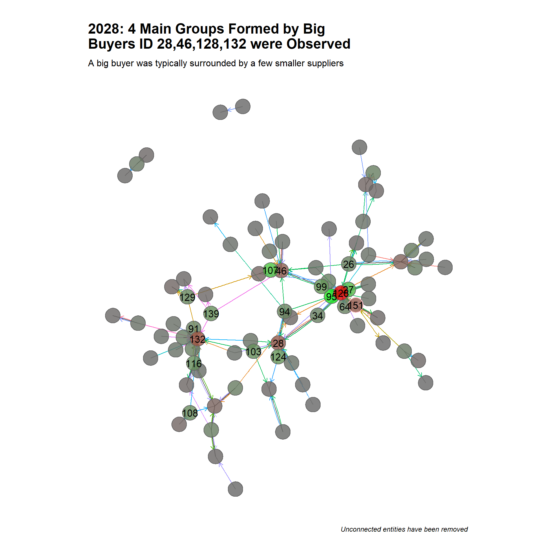
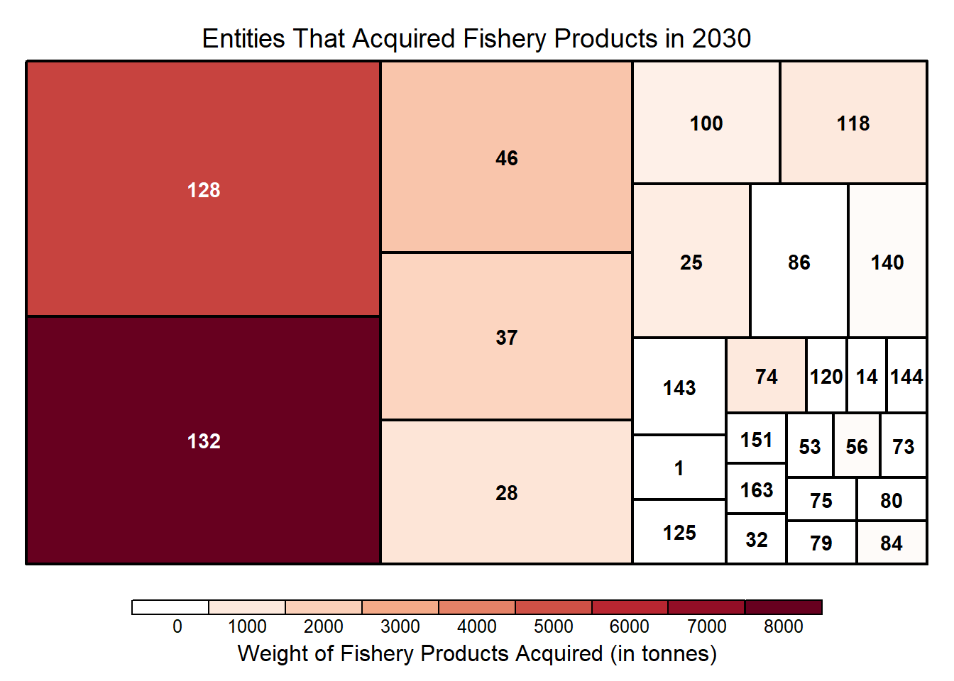
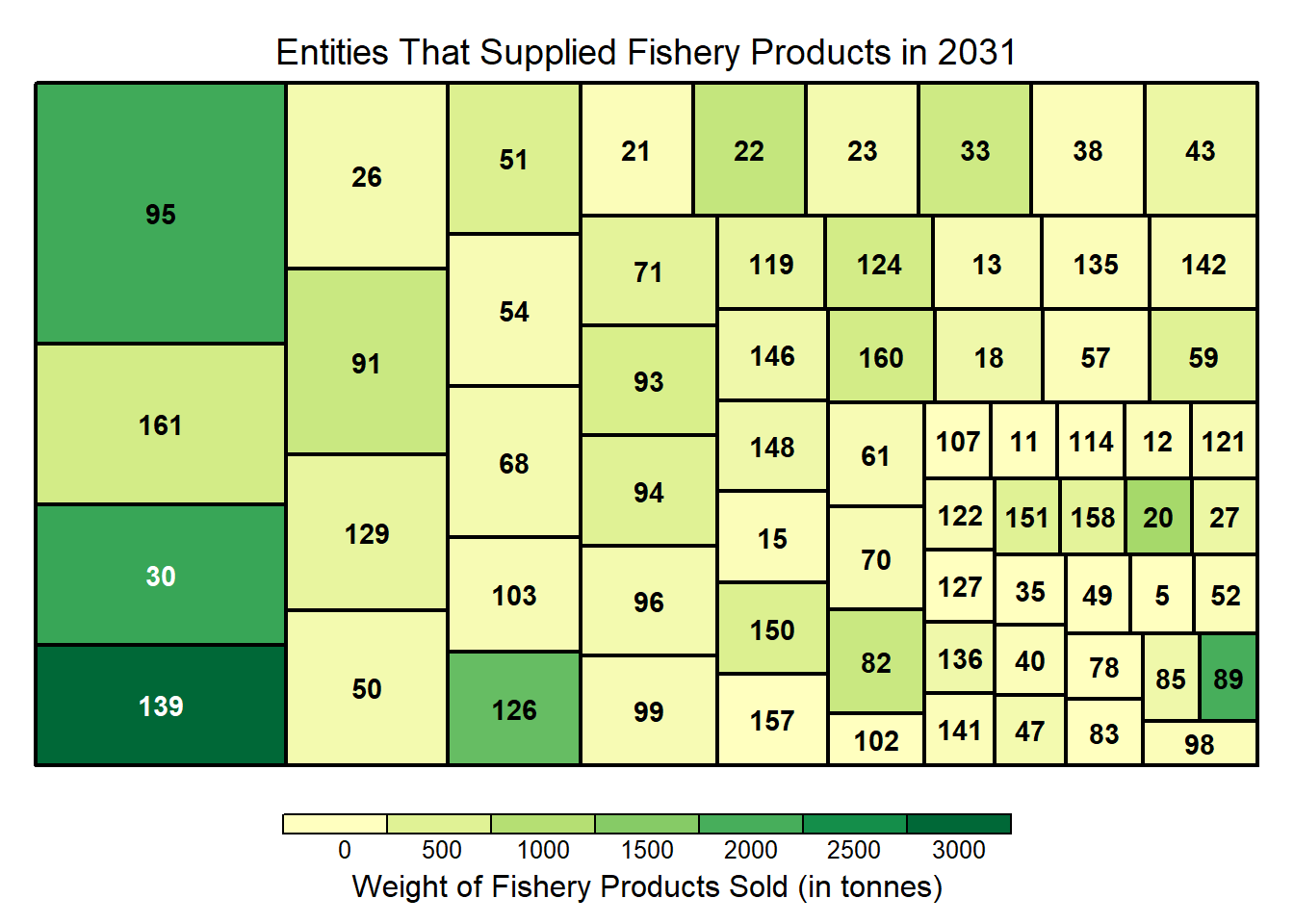
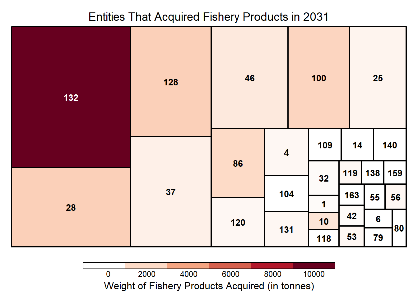
The 4 main buyer groups (or clusters in the networ), lead by ID 28, 46, 128, 132), are probably well-established seafood importers supplying to the Oceanus.
Larger buyers attract larger suppliers and will also acquire from smaller fisheries and vessels.
Re-sellers ID 32 and 84 joined the network, traded actively with many parties and then left the network shortly. ID 84 was dormant in Year 2032 and 2033 and became active again in Year 2034. Given that re-sellers are often associated with transshipping entities and that non-compliant entities often close and open to avoid detection, it is worth further examining and assessing if their trade had been legitimate.
4.Identify the types of business relationship patterns between entities 🈺
The entities in Community ID 14 are categorised into 3 groups: (1) Suppliers (2) Buyers and (3) Re-sellers.
4.1 Main players in each business group
The top 5 sellers in the network based on their out-degree centrality are:
Show the code
n <- 5

nodes_active <- subgraph_obj %>%
  as_tbl_graph() %>%
  activate(nodes) %>%
  mutate(
        in_deg_centrality = round(centrality_degree(weights = weight, mode = "in", loops = FALSE),3),
        out_deg_centrality = round(centrality_degree(weights = weight, mode = "out", loops = FALSE),3),
        out_deg_closeness = round(centrality_closeness(weights=weight,mode='out',normalized = TRUE),3),
        in_deg_closeness = round(centrality_closeness(weights=weight,mode='in',normalized = TRUE),3),
        between_centrality = round(centrality_betweenness(weights = weight, directed = T),3)
        ) %>%
  mutate(
      in_deg_norm = ifelse(in_deg_centrality == 0, 0, (in_deg_centrality - min(in_deg_centrality)) / (max(in_deg_centrality) - min(in_deg_centrality)) + 1),
      out_deg_norm = ifelse(out_deg_centrality == 0, 0, (1 - (out_deg_centrality - min(out_deg_centrality)) / (max(out_deg_centrality) - min(out_deg_centrality))))
    ) %>%
    mutate(combined_in_out_deg = in_deg_norm + out_deg_norm) %>%
  as_tibble()


bigger_suppliers_cnt <- nodes_active %>%
  arrange(desc(out_deg_centrality)) %>%
  select(row_id,id, shpcountry, rcvcountry, out_deg_centrality) %>%
  rename(Name = id,
         ID = row_id) %>%
  top_n(n,wt = out_deg_centrality)

kable(bigger_suppliers_cnt) %>%
  kable_styling(full_width = FALSE) %>%
add_header_above(c("Table 3: Top 5 Suppliers by Frequency" = 5))| ID | Name | shpcountry | rcvcountry | out_deg_centrality |
|---|---|---|---|---|
| 139 | Seashell Seekers LLC Delivery | Marebak | unknown | 859 |
| 95 | Mar del Norte United | Zawalinda | Oceanus | 570 |
| 126 | Rajasthan Marine sanctuary Underwater | Oceanus | Oceanus | 381 |
| 27 | Black Sea Anchovy Pic Wharf | Vesperanda | Oceanus | 269 |
| 124 | Portuguese Sea Bass Ltd. Liability Co | Faraluna | Oceanus | 264 |
The top 5 sellers in the network based on their in-degree centrality are:
Show the code
bigger_buyers_cnt <- nodes_active %>%
  arrange(desc(in_deg_centrality)) %>%
  select(row_id,id, shpcountry, rcvcountry, in_deg_centrality)  %>%
  rename(Name = id,
       ID = row_id) %>%
  top_n(n,wt = in_deg_centrality)

kable(bigger_buyers_cnt) %>%
  kable_styling(full_width = FALSE) %>%
add_header_above(c("Table 4: Top 5 Buyers by Frequency" = 5))| ID | Name | shpcountry | rcvcountry | in_deg_centrality |
|---|---|---|---|---|
| 132 | Sailors and Surfers Incorporated Enterprises | Puerto Sol | Oceanus | 1767 |
| 128 | Rift Valley fishery Inc | Puerto del Mar | Oceanus | 1647 |
| 28 | Black Sea Tuna Sagl | Nalakond | Oceanus | 771 |
| 46 | David Ltd. Liability Co Forwading | Coralada | Oceanus | 543 |
| 37 | Coral Cove BV Delivery | Quornova | Oceanus | 420 |
The top 5 re-sellers in the network based on their betweenness centrality are:
Show the code
bigger_resell_cnt <- nodes_active %>%
  arrange(desc(between_centrality)) %>%
  select(row_id,id, shpcountry, rcvcountry, between_centrality)  %>%
  rename(Name = id,
       ID = row_id) %>%
  top_n(n,wt = between_centrality)

kable(bigger_resell_cnt) %>%
  kable_styling(full_width = FALSE) %>%
add_header_above(c("Table 5: Top 5 Re-sellers by Connectivity Score" = 5))| ID | Name | shpcountry | rcvcountry | between_centrality |
|---|---|---|---|---|
| 84 | Ltd. Liability Co Corp | Coralmarica | Oceanus | 13 |
| 32 | Bu yu wang AG | Zawalinda | Oceanus | 11 |
| 109 | Ocean Oasis S.A. de C.V. Transport | Thessalandia | Oceanus | 11 |
| 119 | Playa Azul Sp Shipping | Arreciviento | Oceanus | 8 |
| 144 | Spanish Anchovy CJSC Marine | Merigrad | Oceanus | 5 |
| 159 | bái suō wěn lú S.p.A. | Syrithania | Oceanus | 5 |
We will take 2 players from the each group to understand their business relationship and trading patterns through an interactive network.
The following visual cue will help us identify their role in the network.
Don’t forget to mouse over the nodes and edges to see the tooltips for more info!
Show the code
# Prepare the edge data set
edges_aggregated <- subgraph_obj %>%
  as_tbl_graph() %>%
  activate(edges) %>%
  as_tibble() %>%
  mutate(title = paste('Count = ',weight,'<br>HSCODE =', short_desc),
         value = weight)
         #value = weight, label = paste(short_desc))


# define grpuping based on the value of combined_in_out_degree

cut_breaks <- c(0, 0.6, 0.9,1.1, 1.4,2)
cut_labels <- c('1 High Out-Degree','2 Medium Out-Degree','3 Low Degree','4 Medium In-Degree','5 High In-Degree' )

nodes_active2 <- nodes_active[,-1] %>%
  mutate(categories=cut(combined_in_out_deg, breaks = cut_breaks, labels = cut_labels, include.lowest = TRUE)) %>%
  mutate(categories = ifelse(between_centrality > 0, "6 Resell\\Tranship", as.character(categories))) %>%
  # Requirement of visNetwork to name grouping column as such
  rename(group = categories) %>%
  mutate(id = row_number()) %>%
  mutate(title = paste(id,label,"<br>Rcv Ctry =", rcvcountry,'<br>Shp Ctry =',shpcountry))

# Plot the intereactive graph
visNetwork(nodes_active2,
           edges_aggregated,
          main = "Transaction graph grouped by Deg centrality intervals",
           height = "500px", width = "100%") %>%
  visIgraphLayout(layout = "layout_nicely") %>%
  #visNodes(shape = 'dot', value = 'pagerank') %>%
  visEdges(arrows = 'to',
           smooth = list(enables = TRUE,
                         type= 'continuous'),
           shadow = FALSE,
           dash = FALSE) %>%
  visOptions(highlightNearest = list(enabled = T, degree = 1, hover = T),
             nodesIdSelection = TRUE,
             selectedBy = "group") %>%
  visGroups(
    groupname = '1 High Out-Degree',
    color = "#20E620")  %>%
  visGroups(
    groupname = '2 Medium Out-Degree',
    color = "#B6D7A8") %>%
  visGroups(
    groupname = '3 Low Degree',
    color = "#666666") %>%
  visGroups(
    groupname = '4 Medium In-Degree',
    color = "#EA9999")  %>%
  visGroups(
    groupname = '5 High In-Degree',
    color = "#E00000")  %>%
  visInteraction(hideEdgesOnDrag = TRUE) %>%
  visLegend(enabled=F) %>%
  visLayout(randomSeed = 123)
4.2 The Bigger Sellers
Big Seller 1: 139, Seashell Seekers LLC Delivery (Seashell)
Business relationship patterns: Supplied fishery products to customers of various sizes, including big buyers such as Sailors and Surfers and Rift Valley fishery Inc.
(Image 1: Direct Trading Network of Seashell)
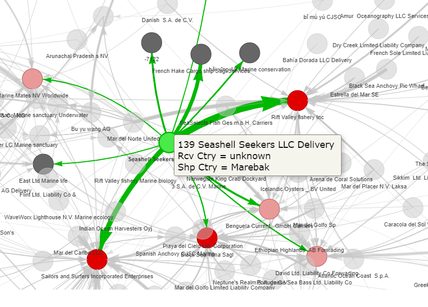
Seashell is a large overseas supplier of various seafood products selling to businesses in Oceanus. As shown in the temporal analysis, Seashell (ID 139) became a significant supplier in the Year 2031 and grew over the years. This corroborates with the EDA observation that there was a surge in transactions in Year 2031.
Volume of Sales (in kg) to customers over the 7 years are as follows:
Show the code
biz <- 'Seashell Seekers LLC Delivery'
id <- 139

# Identity unique customers
unique_customers <- edges_aggregated %>%
  filter(from == id) %>%
  select(from, to) %>%
  inner_join(nodes_active2,select(id,label),by= c('to'='id')) %>%
  select(label) %>%
  unique()

# Identity relevant transactions of customers
edges_customers <- mc2_edges_fish %>%
  filter(source == biz)%>%
  filter(target %in% unique_customers$label)

# Prepare data for plotting heatmap
heatmap <- edges_customers %>%
  mutate(month = floor_date(arrivaldate, unit = "month")) %>%
  group_by(target, month) %>%
  summarise(weight = n(),
            sum_weight_ton = sum(weightkg)/1000) %>%
  arrange(desc(target)) %>%
  ungroup() %>%
  mutate(target2 = ifelse(nchar(target)>40, substr(target, 1, 40),target))

dt_from <- "2028-01-01"
dt_to <- '2034-12-31'

# Plot heatmap
plot <- ggplot(heatmap, aes(x = month, y = reorder(target2, sum_weight_ton), fill = sum_weight_ton)) +
  geom_tile(colour="black", size=0.1, show.legend=F,
            aes(text = paste("Name:", target,
                              "<br>Month:", month,
                              "<br>Count:", weight,
                              "<br>Weight(ton):",sum_weight_ton))) +
  scale_fill_distiller(palette="RdPu",
                       direction = 1) +
  scale_y_discrete(name="", expand=c(0,0))+
  scale_x_date(name="Arrival Date",
               limits=as.Date(c(dt_from, dt_to)),
               expand=c(0,0),date_breaks = "1 year",
               date_labels = "%Y-%m") +
  labs(title= paste0(biz,"'s ", 'Sales by Weight (in tonnes)'),
       subtitle=paste0('Breakdown by Buyers from ',
                       dt_from, ' to ',dt_to)) +
  theme_classic()


#  theme(panel.background = element_rect(fill = "gray"))


ggplotly(plot, tooltip = 'text')
Big Seller 2: 27,Black Sea Anchovy Pic Wharf (Black Sea)
Business relationship patterns: Supplied and traded solely with one big buyer
(Image 2: Direct Trading Network of Black Sea)
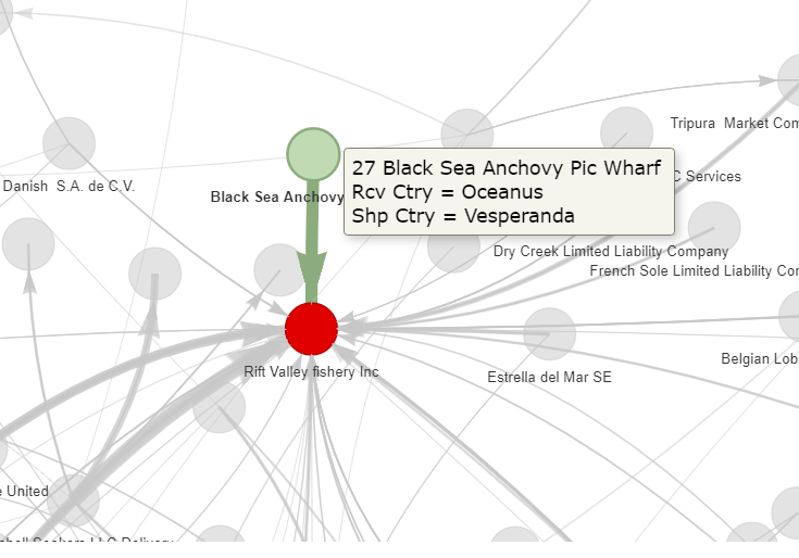
Black Sea’s sole customer in the network was Rift Valley fishery Inc, trading in shrimps and prawns. Black Sea fits the profile of a large fishing vessel or entity, supplying its catches to Rift Valley directly.
4.3 The Bigger Buyers
Big Buyer 1: 132,Sailors and Surfers Incorporated Enterprises (Sailors)
Business relationship patterns: Sourced fishery produce from a large pool of suppliers
(Image 3: Direct Trading Network of Sailors)
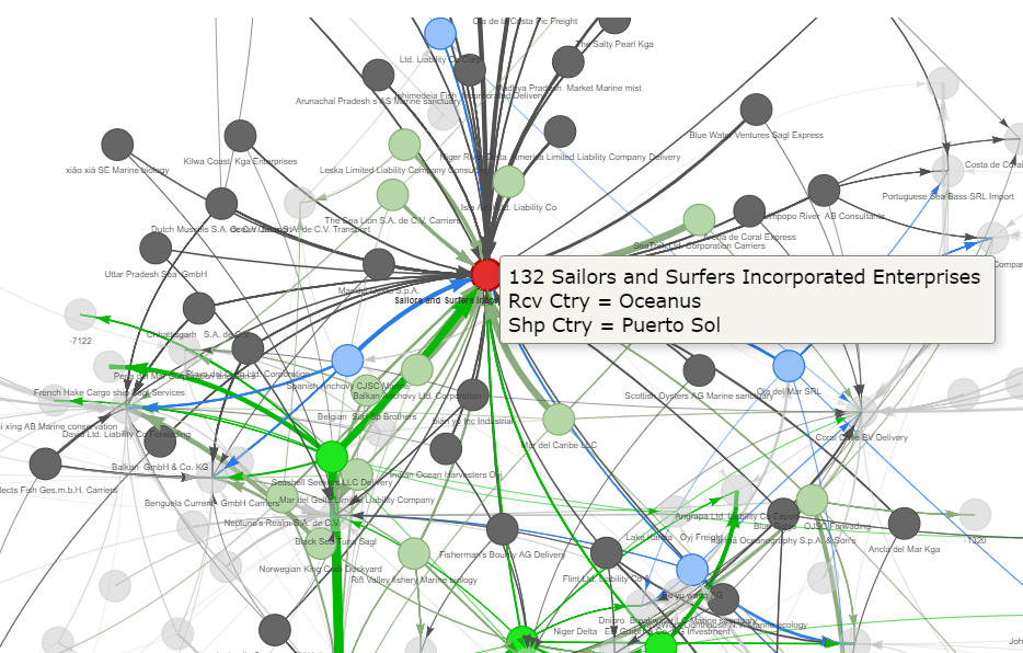
Sailors has been one of the 4 major buyers since Year 2028. It bought various seafood produce, including salmons and hakes. Given these, Sailors is likely a company based in Oceanus importing seafood and buying from local fisheries.
Volume of supplies (in kg) from sellers over the 7 years are as follows:
Show the code
biz <- 'Sailors and Surfers Incorporated Enterprises'
id <- 132

# Identity unique customers
unique_customers <- edges_aggregated %>%
  filter(to == id) %>%
  select(c(from, to)) %>%
  inner_join(nodes_active2,select(id,label),by= c('from'='id')) %>%
  select(c(label)) %>%
  unique()

# Identity relevant transactions of customers
edges_customers <- mc2_edges_fish %>%
  filter(target == biz)%>%
  filter(source %in% unique_customers$label)

# Prepare data for plotting heatmap
heatmap_buy <- edges_customers %>%
  mutate(month = floor_date(arrivaldate, unit = "month")) %>%
  group_by(source, month) %>%
  summarise(weight = n(),
            sum_weight_ton = sum(weightkg)/1000) %>%
  ungroup() %>%
  mutate(source2 = ifelse(nchar(source)>40, substr(source, 1, 40),source))

dt_from <- "2028-01-02"
dt_to <- '2034-12-31'

# Plot heatmap
plot <- ggplot(heatmap_buy, aes(x = month, y = reorder(source2,sum_weight_ton), fill = sum_weight_ton)) +
  geom_tile(colour="White", show.legend=F,
            aes(text = paste("Name:", source,
                              "<br>Month:", month,
                              "<br>Count:", weight,
                              "<br>Weight(ton):",sum_weight_ton))) +
  scale_fill_distiller(palette="Gn",
                       direction = 1) +
  scale_y_discrete(name="", expand=c(0,0))+
  scale_x_date(name="Arrival Date",
               limits=as.Date(c(dt_from, dt_to)),
               expand=c(0,0),date_breaks = "1 year",
               date_labels = "%Y-%m") +
  labs(title= paste0(biz,"'s ", 'Purchases by Weight (in tonnes)'),
       subtitle=paste0('Breakdown by Sellers from ',
                       dt_from, ' to ',dt_to)) +
  theme_classic() +
  theme(legend.position='top',
        plot.title.position="plot",
        axis.text.y=element_text(colour="Black",size=5)) +
  theme(panel.background = element_rect(fill = "gray"))

ggplotly(plot, tooltip = 'text')
From the heatmap, we can see that Sailors ramped up its purchases in Year 2031 when it started to buy from The Sea Lion S.A. de C.V. Carriers and Mar de la Felicidad Co.
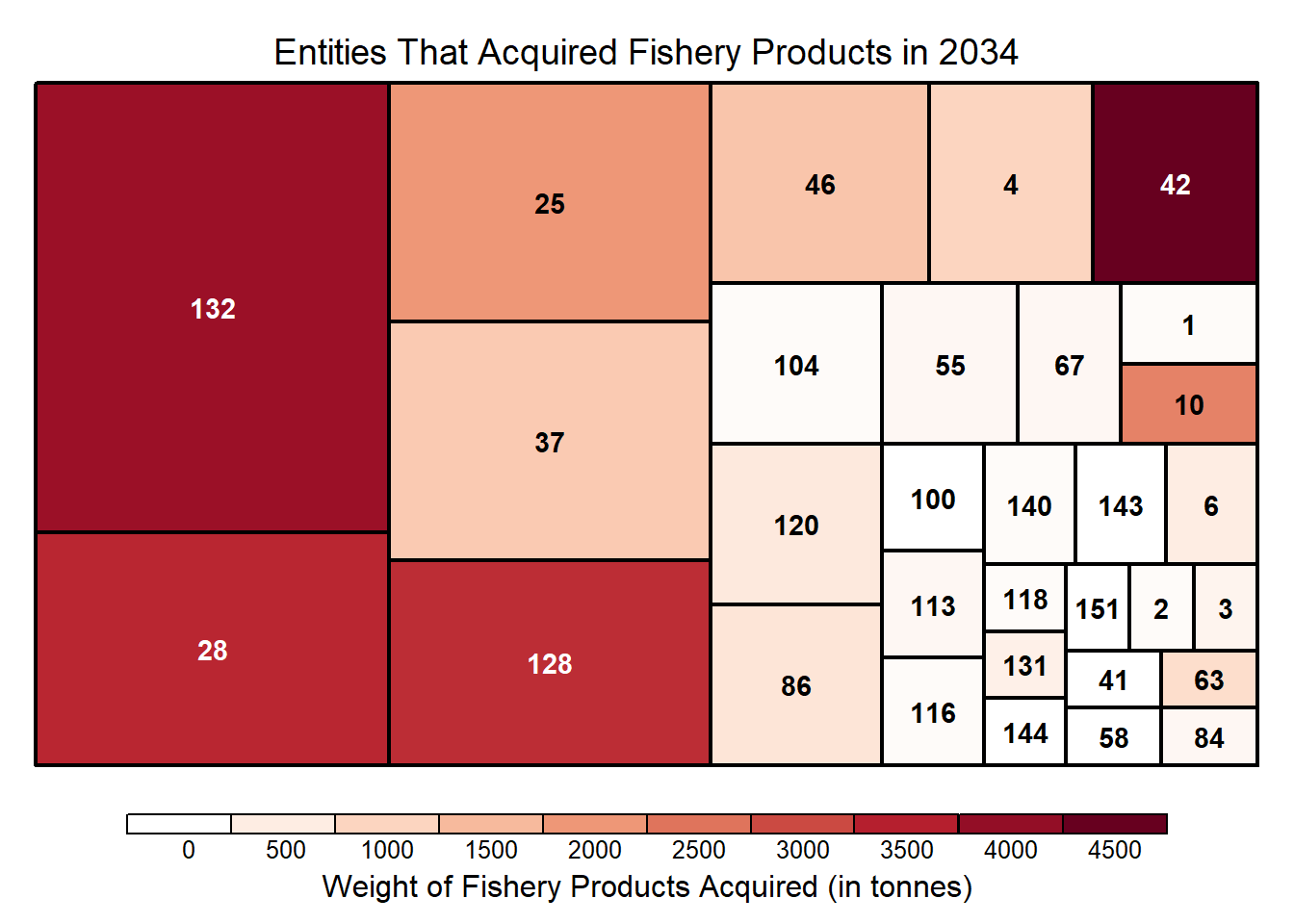
Big Buyer 2: 46,David Ltd. Liability Co Forwading (David)
Business relationship pattern: Bought from a variety of sources, but mainly from smaller suppliers
(Image 4: Direct Trading Network of David)
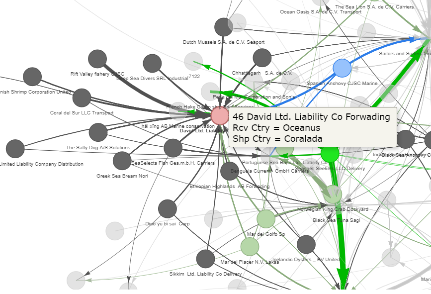
As seen from the image, David sourced its goods and products from a various suppliers, but mainly from smaller suppliers. It traded mainly in fishes as opposed to other types of seafood. From its business name, David was a forwarder; however, this was not apparent from network.
Volume of supplies (in kg) from sellers over the 7 years are as follows:
Show the code
biz <- 'David Ltd. Liability Co Forwading'
id <- 46

# Identity unique customers
unique_customers <- edges_aggregated %>%
  filter(to == id) %>%
  select(c(from, to)) %>%
  inner_join(nodes_active2,select(id,label),by= c('from'='id')) %>%
  select(c(label)) %>%
  unique()

# Identity relevant transactions of customers
edges_customers <- mc2_edges_fish %>%
  filter(target == biz)%>%
  filter(source %in% unique_customers$label)

# Prepare data for plotting heatmap
heatmap_buy <- edges_customers %>%
  mutate(month = floor_date(arrivaldate, unit = "month")) %>%
  group_by(source, month) %>%
  summarise(weight = n(),
            sum_weight_ton = sum(weightkg)/1000) %>%
  ungroup()  %>%
  mutate(source2 = ifelse(nchar(source)>40, substr(source, 1, 40),source))

dt_from <- "2028-01-02"
dt_to <- '2034-12-31'

# Plot heatmap
plot <- ggplot(heatmap_buy, aes(x = month, y = reorder(source2,sum_weight_ton), fill = sum_weight_ton)) +
  geom_tile(colour="White", show.legend=F,
            aes(text = paste("Name:", source,
                              "<br>Month:", month,
                              "<br>Count:", weight,
                              "<br>Weight(ton):",sum_weight_ton))) +
  scale_fill_distiller(palette="Gn",
                       direction = 1) +
  scale_y_discrete(name="", expand=c(0,0))+
  scale_x_date(name="Arrival Date",
               limits=as.Date(c(dt_from, dt_to)),
               expand=c(0,0),date_breaks = "1 year",
               date_labels = "%Y-%m") +
  labs(title= paste0(biz,"'s ", 'Purchases by Weight (in tonnes)'),
       subtitle=paste0('Breakdown by Sellers from ',
                       dt_from, ' to ',dt_to)) +
  theme_classic() +
  theme(panel.background = element_rect(fill = "gray"))

ggplotly(plot, tooltip = 'text')
For David, we will notice that prior to Year 2031, its major suppliers were Norwegian King Crab Dockyard, Rift Valley fishery OJSC and Chhattisgarh S.A. de C.V. The trade relationship with these 3 suppliers stopped from Year 2031 and since then, David appeared to have scaled down its operations and not buying as much as before.
4.4 The Re-sellers with High Connectivity Scores
Reseller 1: 84,Ltd. Liability Co Corp (Ltd)
Business relationship pattern: Traded in various seafood produce as an re-seller
(Image 5: Direct Trading Network of Ltd)
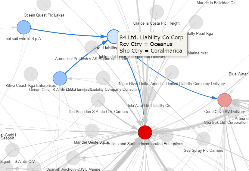
Ltd did not trade with with primary suppliers directly. Instead, it played an intermediary role, acquiring its goods and products from 2 other re-sellers before supplying them to end buyers. In the temporal analysis, we noted that Ltd existed from the community in Year 2032, 3 years after its appearance in Year 2029. Thereafter, it became active again in Year 2034.
Re-seller 2: 144, Spanish Anchovy CJSC Marine (Spanish)
Business relationship pattern: Trader of various seafood produce
(Image 6: Direct Trading Network of Spanish)
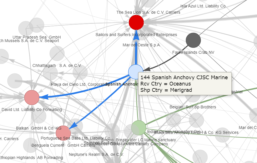
Unlike Ltd, Spanish sourced its goods direct from suppliers acting much like a seasfood trading company or brokerage. Seafood trading companies act as intermediaries between fishing boats, seafood suppliers, and customers. They purchase seafood directly from fishing boats locally and may also source seafood products from overseas suppliers. In addition, seafood trading companies often cater to a wide range of customers, including wholesalers, retailers, restaurants, and other food service providers.
5.Conclusion 🐟
This analysis focuses on a subset of edge transactions that involve live, fresh, chilled, frozen seafood products, based on selected HS codes within a chosen community. By doing so, we focused on and uncovered the trading patterns of various entities and the business models they adopted within the community. Although we found some re-sellers suspicious of being involved in transshipment, it would be premature to conclude that the transactions involved IUU fishing.
Creating meaningful network graphs is a challenging task that requires a lot of time and effort to explore and experiment with different options. However, the benefit is that we can discover patterns that are not easily visible using other types of visualisation.
6.References 🐡
Transshipment Ban Needed to Stop Illegal Fishing and Human Trafficking, Food and Farm Discussion Lab (fafdl.org)
Harshita Kanodia (June 2022), IUU Fishing in the Indian Ocean: A Security Threat. Diplomatist, https://diplomatist.com/2022/06/09/lets-catch-the-big-fish/
Intro to tidygraph and ggraph, Intro to tidygraph and ggraph (jeremydfoote.com)
Jordan Ong Zhi Rong (5-Jun-2022), Take-Home Exercise 6, Take-Home Exercise 6 (isss608-jordan-va.netlify.app)
Wang Xuze (20-Nov-2019), IS428 - DataViz Makeover 2, RPubs - IS428 - DataViz Makeover 2 - Xuze
Options for visNetwork, an R package for interactive network visualisation, Options (datastorm-open.github.io)
Andew J. Park and Stefano Z. Stamato (Andew and Stefano 2020), Social Network Analysis of Global Transshipment: A Framework for Discovering Illegal Fishing, 2020 IEEE/ACM International Conference on Advances in Social Networks Analysis and Mining
P.S. > I would like to express my gratitude to my course instructor who offered invaluable guidance during the analysis process. Also a shout out to my 2 groupmates who provided good ideas to tackle this task.