Countering illegal fishing: Identify anomalies in the business groups

(First Published: Jun 18, 2023)

(Authorities have a challenging task of enforcing on IUU as many fishing companies and owners deliberately exploit a variety of complex company structures, with individual companies based across many jurisdictions, to own and run their operations.)

1. Overview

1.1 Setting the Scene

FishEye International, a non-profit focused on countering illegal, unreported, and unregulated (IUU) fishing, has been given access to an international finance corporation’s database on fishing related companies. In the past, FishEye has determined that companies with anomalous structures are far more likely to be involved in IUU (or other “fishy” business). FishEye has transformed the database into a knowledge graph. It includes information about companies, owners, workers, and financial status. FishEye is aiming to use this graph to identify anomalies that could indicate a company is involved in IUU.

1.2 Our Task

In response to Question 1 of VAST Chaellenge 2023: Mini-Challenge 3, our task is to use visual analytics to identify anomalies in the business groups present in the given knowledge graph.

2.Set Up

2.1 Load the relevant packages into the R environment

We use the pacman::p_load() function to load the required R packages into our working environment. The loaded packages are:

• igraph : provides functions for creating, analyzing, and visualizing graphs

• tidygraph : provides a tidy and consistent way to work with graph data structure

• ggraph : creates visualizations of graphs using the grammar of graphics approach

• ggforce : provides additional geoms, stats, and scales to enhance the capabilities of ggplot2

• visNetwork : creates interactive network visualizations

• tidyverse : a collection of packages in R that work together to provide a consistent and coherent approach to data manipulation and analysis

• jsonlite : for working with JSON (JavaScript Object Notation) data

• plotly : for creating interactive web-based graphs

• knitr: for dynamic report generation

• kableExtra : provides additional customization options for tables created with the knitr package,

• skimr : provides summary statistics and visualizations for exploring and understanding data

• DT : creates interactive tables using the DataTables JavaScript library

• tidytext : focuses on text mining and natural language processing (NLP) tasks

• textstem : offers stemming algorithms for text analysis

• ggiraph : adds interactivity to ggplot2 visualizations

Show the code

pacman::p_load(igraph, tidygraph, ggraph, ggforce, visNetwork, tidyverse, jsonlite, plotly, knitr, kableExtra, skimr, DT,tidytext, textstem, ggiraph)

# Set the default display settings for numeric values to see large numbers in full
options(scipen = 999, digits = 15)

2.2 Import and Extract the data

The given data is an undirected knowledge graph provided in json format. It contains 2 sets of information - Nodes and Edges attributes .

1. First, we imported the data and assigned it to a variable mc3.

Show the code

mc3 <- fromJSON("data/mc3.json")

2. Next, we extracted the nodes data frame from mc3.

At the same time, we applied distinct() to remove duplicate node records and rounded the revenue_omu values to the nearest whole unit so that it would be easier for us to work with the attribute given its small denomination .

Show the code

# Extract the nodes data

# convert the fields to characters first to extract the information embedded as list
mc3_nodes <- as_tibble(mc3$nodes) %>%
  # mutate() and as.character() are used to convert the field data type from list to character
  mutate(country = as.character(country),
         id = as.character(id),
         product_services = as.character(product_services),
         revenue_omu = as.numeric(as.character(revenue_omu)),
         type = as.character(type)) %>%
  # Re-organise the columns
  select(id,country,type,product_services,revenue_omu) %>%
  # remove duplicate records
  distinct() %>%
  # omu is denominated in smaller currency units, so we will round all values to the nearest whole unit to make it easier to work with
  mutate(revenue_omu = round(revenue_omu,0)) 

3. Then, we extracted the edges data frame from mc3.

Show the code

# Extract the edge data
mc3_edges <- as_tibble(mc3$links) %>%
  # remove the duplicates
  distinct() %>%
  #mutate() and as.character() are used to convert the field data type from list to character
  mutate(source = as.character(source),
         target = as.character(target),
         type = as.character(type)) %>%
  group_by(source, target, type) %>%
  summarise(weight = n()) %>%
  # Included to ensure self-links are excluded, although there was none found
  filter(source!=target) %>%
  ungroup

Observations

• Although we included distinct() function to remove duplicate records in the codes above, there was no such records or self-links

• Grouping by source, target and type did not reduce the number of records, and the weight for all records show 1. This meant the edge information contain the relationships between the entities involved and might not connote the volume of transactions between them

We stored the extracted mc3 nodes and edges data frames in rds format for ease of subsequent retrieval. The following “write” code lines need only be executed once. Thereafter we can reload the mc3_nodes and mc3_edges data frames for data wrangling.

Show the code

# write and load the mc3_nodes and edges dataframe. With this, we need not re-extract from the raw dataset subsequently

#write_rds(mc3_nodes, "data/mc3_nodes.rds")
mc3_nodes = read_rds("data/mc3_nodes.rds")

#write_rds(mc3_edges, "data/mc3_edges.rds")
mc3_edges <- read_rds("data/mc3_edges.rds")

2.3 Data Preparation

2.3.1 The Edges data frame

1. We started data perpetration by inspecting the mc3_edges data frame using skim()

Show the code

skim(mc3_edges)

Data summary

Name	mc3_edges
Number of rows	24036
Number of columns	4
_______________________
Column type frequency:
character	3
numeric	1
________________________
Group variables	None

Variable type: character

skim_variable	n_missing	complete_rate	min	max	empty	n_unique	whitespace
source	0	1	6	700	0	12856	0
target	0	1	6	28	0	21265	0
type	0	1	16	16	0	2	0

Variable type: numeric

skim_variable	n_missing	complete_rate	mean	sd	p0	p25	p50	p75	p100	hist
weight	0	1	1	0	1	1	1	1	1	▁▁▇▁▁

Observations

• There was no field with missing value

• There were 2 unique relationship types: Entity - Beneficial Owner (BO), Entity - Company Contact (CC). We assumed that the source entities were companies, the target entities were all individuals associated with the companies and their relationships were reflected under type column.

• The source column has a maximum length of 700 characters, which was atypical of most entity names. This was examined in the next step.

2. We then examined records with lengthy text in the source column

We pulled out some records with more than 100 characters in the source column.

Show the code

# Set variable n for character limit 
n <- 100

# filter such records
filtered_data <- mc3_edges %>%
  filter(str_length(source) > n)
 

# Inspect the filtered records
kable(head(filtered_data, n=5)) %>%
  kable_styling(full_width = FALSE) %>%
  add_header_above(c("Table 1: Sample Records under the Source column with > 100 characters" = 4))

Table 1: Sample Records under the Source column with > 100 characters
source	target	type	weight
c("1 Swordfish Ltd Solutions", "1 Swordfish Ltd Solutions", "Saharan Coast BV Marine", "Olas del Sur Estuary")	Daniel Reese	Company Contacts	1
c("Adriatic Squid Ltd. Liability Co", "Brisa del Este Cargo Bonito", "Sea Harvest Marine conservation CJSC Marine")	Angelica Wheeler	Beneficial Owner	1
c("Adriatic Squid Ltd. Liability Co", "Brisa del Este Cargo Bonito", "Sea Harvest Marine conservation CJSC Marine")	Shelly Strong	Company Contacts	1
c("Ancla Azul ОАО Holdings", "Ancla Azul ОАО Holdings", "Ancla Azul ОАО Holdings", "Playa de Arena Sagl")	Jennifer Morales	Company Contacts	1
c("Ancla del Este OJSC", "Irish Trout S.p.A. Carriers", "Irish Trout S.p.A. Carriers", "Irish Trout S.p.A. Carriers", "Irish Trout S.p.A. Carriers", "Irish Trout S.p.A. Carriers")	Carlos Harvey	Company Contacts	1

We noticed that these rows contain list of entities in the source column, implying that there were records with many source entities to one single target entity. To flatten the records, we extracted and then converted such rows from the edge data frame to additional link records using the separate_rows() function to split each element in the embedded list into a separate row while repeating the values in other columns.

Show the code

# Extract records with lists in source column
filtered_data_list <- mc3_edges%>%
  # filter records starting with 'c("' in the source column
  filter(str_starts(source, '^c\\("')) %>%
  # remove the first 2 character and last character of the source column
  mutate(source = substr(source, 3, nchar(source) - 1)) %>%
  # split each element in the list in source column to a new row
  separate_rows(source, sep = ",") %>%
  # remove empty string at the start of the source columns
  mutate(source = trimws(source)) %>%
  # remove the opening and closing quotes from the source column
  mutate(source = substr(source, 2, nchar(source) - 1))

# Inspect the filtered records
kable(slice(filtered_data_list, 3:6)) %>%
  kable_styling(full_width = FALSE) %>%
  add_header_above(c("Table 2: Extracted Edge records based on the 1 st record from Table 1" = 4))

Table 2: Extracted Edge records based on the 1 st record from Table 1
source	target	type	weight
1 Swordfish Ltd Solutions	Daniel Reese	Company Contacts	1
1 Swordfish Ltd Solutions	Daniel Reese	Company Contacts	1
Saharan Coast BV Marine	Daniel Reese	Company Contacts	1
Olas del Sur Estuary	Daniel Reese	Company Contacts	1

After we had flattened the records with embedded list in the source column, we combined these processed edge records with those records which did not have any embedded list in the source column originally.

Show the code

# Extract records which had list in their source column
filtered_data <- mc3_edges %>%
  filter(str_starts(source, '^c\\("'))

# Extact records which did not have  any list in the source column originally
remaining_data <- mc3_edges %>%
  anti_join(filtered_data)

# Union remaining_data and desired_rows
mc3_edges_flat <- bind_rows(remaining_data, filtered_data_list) %>%
  # group to eliminate duplicate source, target, type records
  group_by(source,target,type) %>%
  mutate(weight=sum(weight)) %>%
  ungroup() %>%
  # remove repeated rows after grouping
  distinct()

3. Next, we visualised the count of edge records by type

Show the code

mc3_edges_flat %>%
  group_by(type) %>%
  summarise(count = n()) %>%
  ggplot(aes(x = type, y = count)) +
  geom_bar(stat = "identity", fill = "lightblue") +
  geom_text(aes(label = format(count,big.mark=",")), vjust = -0.5) +
  theme_minimal() +
  labs(x = "Edge Type", y = "No. of\nTransactions",
       title = 'Count of Relationships by Type',
       subtitle = "Beneficial Owners accounted for the majority of the edge types") +  # Add the subtitle
  theme(axis.title.y = element_text(angle = 0, vjust = 0.5, hjust = 1)) +
  ylim(0, 20000)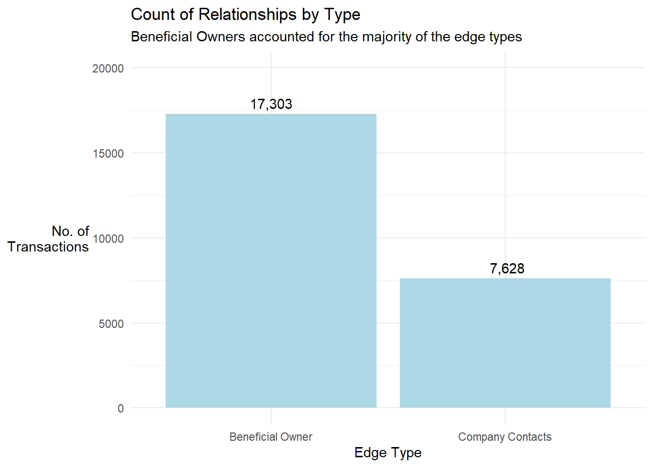 

4. We prepared the nodes data frame using records from the edges data frame

(i) We extracted and combined the entities listed in the source and target columns into an id column. For the target entities, we retained edge type information based on the provided edge records since it was the role of the target entity. For the the source entities, we defaulted their type as Company (this has been discussed in the observation note to Step 1 above). The process resulted in 35,386 unique (id, type) pairs.

Show the code

# Prepare the nodes information using the source and target information in the edge data frame
id1 <- mc3_edges_flat %>%
  select(source) %>%
  mutate(type = "Company") %>%
  rename(id = source)
  
id2 <- mc3_edges_flat %>%
  select(target, type) %>%
  rename(id = target)

# Get unique nodes from source and target columns of edge records
mc3_nodes_fr_edges <- rbind(id1, id2) %>%
  distinct()

(ii) Next, we left joined the mc3_nodes_fr_edges with the mc3_nodes data frame by id and type to get more information about the entities. The information was stored in the mc3_nodes_combined data frame.

Show the code

# Get unique nodes from source and target columns of edge records
mc3_nodes_combined <- left_join(mc3_nodes_fr_edges, mc3_nodes, by = c("id", "type"))

Observations

• The number of node records increased from 35,386 to 35,806. This meant that there were duplicate node records with same id and type (but have different country, revenue_omu or product_services data) in the mc3_nodes dataframe. We further treated these records in Section 2.3.2.
• The left join step above also meant entity records from the mc3_nodes data frame that did not have a matching type would be excluded in our subsequent analysis.

5. Quick visualisation of the network for nodes with high Betweenness Centrality

(i) We computed centrality measures of the nodes. To limit the number of entities to be displayed, we extracted those with Betweenness Centrality scores of >= 100,000.

Show the code

# compute the centrality measures for nodes
mc3_graph <- tbl_graph(nodes = mc3_nodes_combined,
                       edges = mc3_edges_flat,
                       directed = FALSE) %>%
  mutate(betweenness_centrality = centrality_betweenness(),
         closeness_centrality = centrality_closeness())

# set random seed for consistency
set.seed(123)

# plot the graph
mc3_graph %>%
  # we only plot nodes with high betweeness_centrality
  filter(betweenness_centrality >= 100000) %>%
ggraph(layout = "fr") +
  geom_edge_link(aes(alpha=0.5)) +
  geom_node_point(aes(
    linewidth = betweenness_centrality,
    alpha = 0.5)) +
  scale_size_continuous(range=c(0.01,0.5))+
  theme_graph() +
  labs(title = "Initial Network Plot based on Edge Data")+
  theme(legend.position = "none")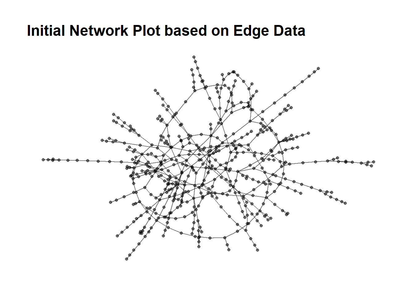

2.3.2 The Nodes data frame

1. Status Check

After performing Step 4(ii) of Section 2.3.1 above, there were entities in the mc3_nodes_combined data frame with > 1 record.

2. We aggregated information of entities with multiple records in the mc3_nodes_combined data frame such that there was only 1 node record per entity.

This was achieved by the following steps:

i. For records with same id, type and country information

We concatenated the product_services information across different rows and sum up their revenue_omu information. This was on the assumption that a company only has 1 record per country.

ii. For records with the same id and type information

We concatenated the country information and also tracked the count of countries involved. We tracked companies with presence in multiple countries as this did not appear to be the norm for the data set.

Show the code

# Step 2(i)
# Identify records with same id and type information
result <- mc3_nodes_combined %>% 
  filter(duplicated(mc3_nodes_combined[, c("id", "type")]) | duplicated(mc3_nodes_combined[, c("id", "type")], fromLast = TRUE))

# Concatenate text values in product_services and sum revenue_omu for records with the same id, type, and country
result_same_coy <- result %>%
  group_by(id, type, country) %>%
  summarize(product_services = paste(product_services, collapse = ", "),
            revenue_omu = sum(revenue_omu)) %>%
  ungroup()

# Step 2(ii)
# Arrange alphabetically in the country column, then concatenate text values for records with the same id, type
result2 <- result_same_coy %>%
  arrange(country) %>%
  group_by(id, type) %>%
  summarize(country = paste(country, collapse = ", "),
            country_count = n(),
            product_services = paste(product_services, collapse = ", "),
            revenue_omu = sum(revenue_omu))

3. We removed records with duplicate Ids from the mc3_nodes_combined data frame and combined the aggregated node records in Step 2 back with mc3_nodes_combined data frame. There were 35,386 unique (id,type) pairs, the same number we got from the m3_edge data frame in Step 4(i) of Section 2.3.1.

Show the code

mc3_nodes_cleaned <- mc3_nodes_combined %>%
  anti_join(result) %>%
  mutate(country_count = 1)
  
mc3_nodes_cleaned <- bind_rows(mc3_nodes_cleaned , result2)  

4. Finally, we aggregated the entities by their Id, resulting in 34,422 unique entity records.

The following logic were applied during the aggregation for rows with same id:

• The node type , country and product_services values were concatenated across rows

• type_count was created to track the number of node types

• The country_count and revenue_omu values were sum-up across rows

Show the code

mc3_nodes_cleaned <- mc3_nodes_cleaned %>%
  arrange(type,country,product_services) %>%
  group_by(id) %>%
  summarize(type = paste(type,collapse =", "),
            type_count = n(),
            country = paste(country, collapse = ", "),
            country_count = max(country_count),
            product_services = paste(product_services, collapse = ", "),
            revenue_omu = sum(revenue_omu)) %>%
  # clean up the country and product_services column after concatenation
  mutate(country = ifelse(country %in% c('NA',"NA, NA"), NA, country),
         product_services = ifelse(product_services %in% c('NA',"NA, NA"), NA, product_services))

5. We visualised the count of node records by type

Show the code

mc3_nodes_cleaned %>% 
  group_by(type) %>%
  summarise(count = n()) %>%
  ggplot(aes(x = type, y = count)) +
  geom_bar(stat = "identity", fill='lightblue') +
  geom_text(aes(label = format(count,big.mark=",")), vjust = -0.5) +
  theme_minimal() +
  labs(x = "Node Type", y = "No. of\nEntities",
       title = 'Count of Nodes by Type',
       subtitle ='There were individuals who had roles as Benenficial Owners and Company Contacts') +
  theme(axis.title.y = element_text(angle = 0, vjust = 0.5, hjust = 1)) +
  ylim(0, 15000)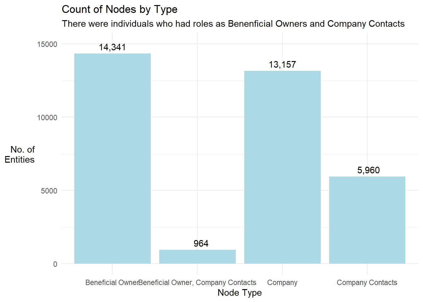 

6. We also visualised the Top 8 countries where the nodes were domiciled in

Show the code

mc3_nodes_cleaned %>%
  filter(!is.na(country)) %>%
  group_by(country) %>%
  summarise(count = n()) %>%
  top_n(10) %>%
  arrange(desc(count)) %>%
  ggplot(aes(x = reorder(country, -count), y = count)) +
  geom_bar(stat = "identity", fill = '#3498db') +
  geom_text(aes(label = format(count,big.mark=",")), vjust = -0.5) +
  theme_minimal() +
  labs(x = "Country", y = "No. of\nNodes",
       title = 'Count of Nodes by Country',
       subtitle = 'Oceanus, Marebak and ZH were the top 3 countries where most nodes domiciled') +
  theme(axis.title.y = element_text(angle = 0, vjust = 0.5, hjust = 1))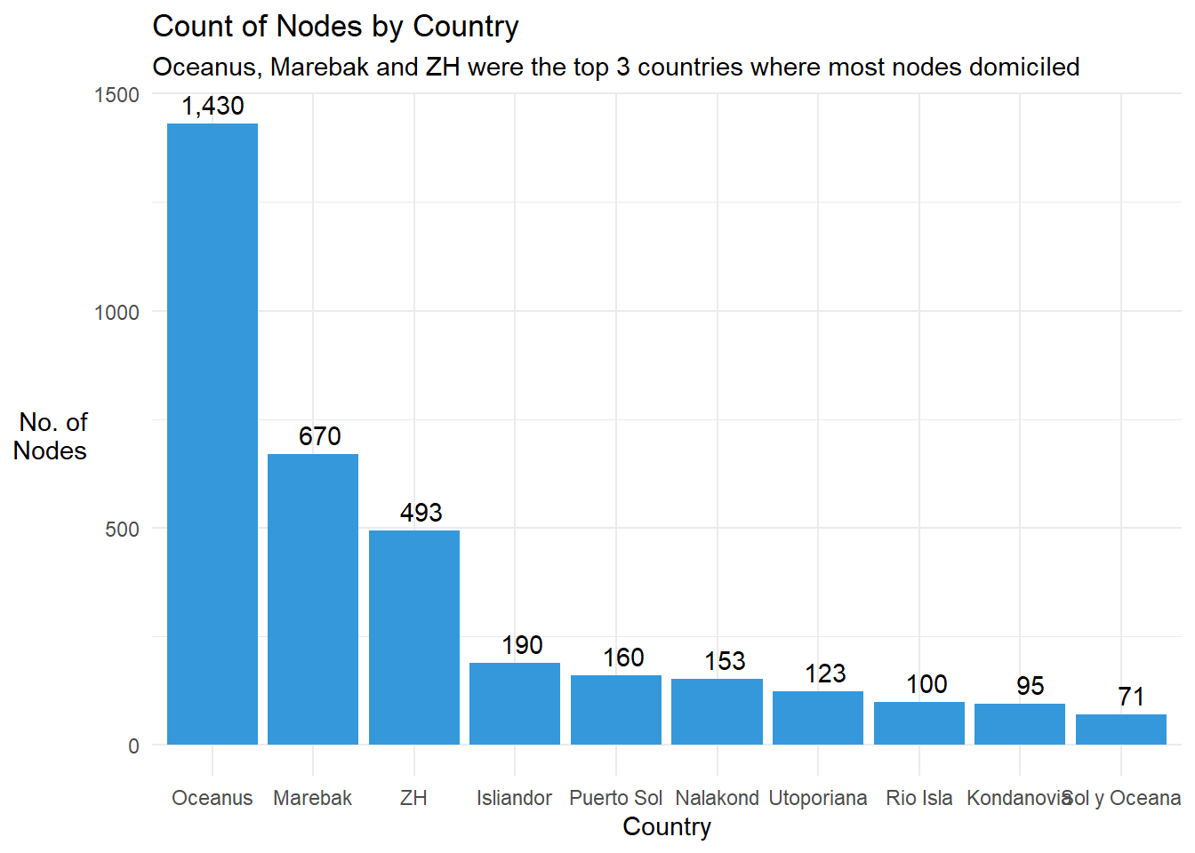 

7. We noticed that values for the product_services column were very different across rows and decided to check the frequency of each value.

Show the code

# Get the freq count of records by product_services column 
freq_count_pdt_svcs <- mc3_nodes_cleaned %>% 
  group_by(product_services) %>%
  summarise(count = n()) %>%
  arrange(desc(count))

datatable(freq_count_pdt_svcs, class = "compact", options = list(pageLength = 5), 
              caption = "Table 3: Frequency Count of Values in product_services Column",
              rownames = FALSE)

Show 5102550100 entries

Search:

Table 3: Frequency Count of Values in product_services Column

product_services	count
	29833
Unknown	2010
Unknown, Unknown	58
Fish and seafood products	36
Seafood products	29

Showing 1 to 5 of 2,148 entries

Previous12345…430Next

8. We saw from the there was a large number of the records with empty strings . “Unknown” or “Unknown, Unknown”. The last category was due to the concatenation we did earlier to aggregate the information for nodes with multiple records. We re-coded “Unknown” and “Unknown, Unknown” to NA.

Show the code

mc3_nodes_cleaned2 <- mc3_nodes_cleaned %>%
  mutate(product_services = trimws(product_services))%>%
  mutate(product_services = replace(product_services, product_services == "Unknown", NA)) %>%
  mutate(product_services = replace(product_services, product_services == "Unknown, Unknown", NA))

2.4 Categorise Entities by their products and services

There were still round 2,170 different types of product and services that the entities offered. The information within the product_services column were highly varied and we performed text sensing to identify entities in the fishing industry, which was the industry of interest for us.

1. Tokenised the words used under the product_services column

Show the code

token_nodes <- mc3_nodes_cleaned2 %>%
  unnest_tokens(word, 
                product_services)

2. Removed common words that did not have much differentiating power

Show the code

# Inclded our own list of stopwords
stopwords = c(NA,'products','services','unknown','related','canned')

# Remove stopwords
stopwords_removed <- token_nodes %>% 
  # Remove default stopwords from tidytext
  anti_join(stop_words) %>%
  # Exclude common words that we defined above
  filter(!word %in% stopwords)

3. Performed lemmatisation to convert all words to their root form

Show the code

stopwords_removed <- stopwords_removed %>%
  mutate(word = lemmatize_words(word))

4. Visualised the frequency count of the words

Show the code

stopwords_removed %>%
  count(word, sort = TRUE) %>%
  top_n(15) %>%
  mutate(word = reorder(word, n)) %>%
  ggplot(aes(x = word, y = n)) +
  geom_col(stat = "identity",fill="#6baed6") +
  geom_text(aes(label = n), vjust = 0.4, hjust=-0.1) +
  xlab(NULL) +
  coord_flip() +
      labs(x = "Count",
      y = "Unique words",
      title = "Count of unique words found in product_services field",subtitle = 'Words relating to fish and seafood produce were prominent') +
  theme_minimal() +
  theme(axis.title.y = element_text(angle = 0, vjust = 0.5, hjust = 1))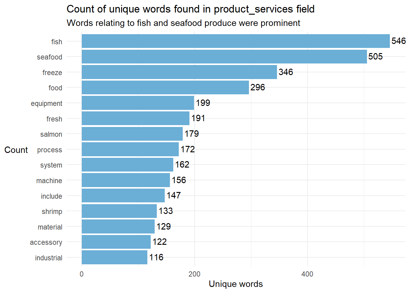

5. We generated a word_count table and exported it to manually identify keywords of various industries for manual categorization. This helped to ensure that we could capture words related to the fishing industry more accurately.

Show the code

# Append a cummulative count column into the stopwords_removed data frame
word_count <-stopwords_removed %>%
  count(word, sort = TRUE) %>%
  mutate(cumulative_percent = cumsum(n) / sum(n) * 100)

# Export the word_count list to csv
# write_csv(word_count,"data/word_count.csv")

Observations

• There were 4,700 unique words

• The first 700 unique words covered 70% of all the text used under the product_servcies column.

6. Through manual inspection of the first 700 most frequent words, we identified the following list of seafood related terms

’fish, seafood, salmon, shrimp, fillet, crab, tuna, shellfish, squid, cod, clam, pollock, lobster, octopus, oyster, scallop, sockeye, crustacean, mackerel, roe, mollusk, mussel, groundfish, cuttlefish, rockfish, caviar, eel, haddock, crayfish, sardine, seabass, catfish, finfish, mollusc, trout”

7. We also identified some keywords to categorise other businesses.

Although this approach was mechanical and not the most comprehensive, it would help the us gain a quick understanding of the business activities of the entity. The 9 main business activities identified were: (i) seafood, (ii) fruits, vegetables and other food, (iii) machinery and equipment, (iv) consumer goods, (v) meat and dairy, (vi) freight and transport, (vii) energy and fuel, (viii) metals, and (ix) chemical and plastic.

Show the code

# Group the prossed words in Step 3 by id
# The tokenised words, separated by commas, for each entity is now appended in product_services2 column
processed_text <- stopwords_removed %>%
  group_by(id) %>%
  summarize(product_services2 = paste(word, collapse = ", "))

# left join mc3_nodes_cleaned2 with the processed text
mc3_nodes_cleaned2 <- left_join(mc3_nodes_cleaned2, processed_text, by = c("id"))

# create list of keywords to identify various businesses

seafood <- as.list(c('fish', 'seafood', 'salmon', 'shrimp', 'fillet', ' crab', ' tuna', 'shellfish', 'squid', ' cod', 'clam', 'pollock', 'lobster', 'octopus', 'oyster', 'scallop', 'sockeye', 'crustacean', 'mackerel', ' roe', 'mollusk', 'mussel', 'groundfish', 'cuttlefish', 'rockfish', 'caviar', ' eel', 'haddock', 'crayfish', 'sardine', 'seabass', 'catfish', 'finfish', 'mollusc'))

fruits <- as.list(c('food', 'fruit', 'vegetable', 'vegetables', 'tomato',' gelatine','gelatin','salt','coffee'))

machinery <- as.list(c('equipment', 'machine', 'machinery', 'automation'))
consumer <- as.list(c('accessory', 'fabric', 'adhesive', 'paper', 'clothing', 'stationery', 'toy', 'yarn', 'dress', 'pencil', 'shirt', 'pens',' 
footwear','workwear',   'apparel','footwear','shoe','sandal','bag','grocery'))

meat <-as.list(c('meat', 'steak', 'milk', 'poultry', 'beef', 'chicken', 'pork', 'lamb', 'dairy'))
freight <- as.list(c('freight', 'transportation', 'logistic', 'cargo', 'transport', 'warehouse', 'shipping', 'truck', 'trucking', 'forwarding','boat charter','automobile'))

energy <- as.list(c('oil', 'gas', 'energy','electricity'))

metals <- as.list(c('metal', 'steel', 'aluminum','aluminium', 'copper', 'alloy', 'metals'))

chemicals <- as.list(c('chemical','plastic','ammonia'))

# Create a new column 'category' and assign the entity to a industry based on the keywords defined above
mc3_nodes_cleaned3 <- mc3_nodes_cleaned2 %>%
  mutate(category = "other") %>%
  mutate(category = if_else(str_detect(product_services2, paste(fruits, collapse = "|")), "fruits, vegetables and other food", category)) %>%
  mutate(category = if_else(str_detect(product_services2, paste(machinery, collapse = "|")), "machinery and equipment", category)) %>%
  mutate(category = if_else(str_detect(product_services2, paste(consumer, collapse = "|")), "consumer goods", category)) %>%
    mutate(category = if_else(str_detect(product_services2, paste(meat, collapse = "|")), "meat and dairy", category)) %>%
    mutate(category = if_else(str_detect(product_services2, paste(freight, collapse = "|")), "freight and transport", category)) %>%
      mutate(category = if_else(str_detect(product_services2, paste(energy, collapse = "|")), "energy and fuel", category)) %>%
      mutate(category = if_else(str_detect(product_services2, paste(metals, collapse = "|")), "metals", category)) %>%
        mutate(category = if_else(str_detect(product_services2, paste(chemicals, collapse = "|")), "chemical and plastic", category)) %>%
  # Seafood category was placed last to override earlier categorisation
  mutate(category = if_else(str_detect(product_services2, paste(seafood, collapse = "|")), "seafood", category))

8. Performed a frequency code to find out the number of entities categorised as seafood

Show the code

freq_industry <- mc3_nodes_cleaned3 %>%
  filter(!is.na(category)) %>%
  group_by(category) %>%
  summarise(count = n(),
            total_revenue =format(sum(revenue_omu, na.rm=TRUE), big.mark=","),
            avg_revenue = format(round(mean(revenue_omu, na.rm=TRUE),0), big.mark=",")
            ) %>%
  arrange(desc(count)) %>%
  ungroup()


# Inspect the filtered records
kable(freq_industry) %>%
  kable_styling(full_width = FALSE) %>%
  add_header_above(c("Table 4: Frequency Count and Revenue of Entities By Industry" = 4))

Table 4: Frequency Count and Revenue of Entities By Industry
category	count	total_revenue	avg_revenue
seafood	694	225,860,850	388,077
other	567	556,995,019	1,218,807
consumer goods	331	211,739,917	778,456
freight and transport	187	421,253,488	2,632,834
fruits, vegetables and other food	160	33,876,949	245,485
chemical and plastic	156	279,194,590	2,215,830
metals	152	59,611,880	518,364
machinery and equipment	142	84,695,891	730,137
energy and fuel	64	114,295,659	2,241,091
meat and dairy	60	33,166,401	637,815

Observations

• Seafood industry had the most number of entities and the avearge revenue per entity was the second lowest (after fruits, vegetables and other food) among the 9 industry sectors featured.

3.Identify business groups with anomalies

We were informed that companies with anomalous structures are far more likely to be involved in IUU (or other “fishy” business). Hence, we looked into the following aspects of structural anomalies from among the seafood business groups:

1. Business Groups with high network diameter
2. Business Groups with with exceptional business revenue
3. Business Groups that operated across multiple countries

For our analysis, we defined a business group as one that had at least one seafood entity in a connected network.

3.1 Business Groups with high network diameter

1. To identify the relevant business groups with at least 1 seafood entity, we extracted the seafood_nodes and edge records of seafood entities for network examination

Show the code

# extract the entities categorised as seafood
seafood_entities <- mc3_nodes_cleaned3 %>%
  filter(category=='seafood')

# extract the edge link records related to these seafood entities
seafood_edges <- mc3_edges_flat[mc3_edges_flat$source %in% seafood_entities$id | mc3_edges_flat$target %in% seafood_entities$id, ]

# extract the seafood_nodes records using the edge information
id1 <- seafood_edges %>%
  select(source) %>%
  rename(id = source)
  
id2 <- seafood_edges %>%
  select(target) %>%
  rename(id = target)

# Get unique nodes from source and target columns of edge records
# left join with the mc3_nodes_cleaned3 dataset to get the attributes for the nodes
seafood_nodes <- rbind(id1, id2) %>%
  distinct() %>%
  left_join(mc3_nodes_cleaned3,by=c('id'))

2. Next, we prepared the tbl_graph object for network computation and plotting

Show the code

seafood_graph<- tbl_graph(nodes=seafood_nodes,
                          edges = seafood_edges,
                          directed = FALSE)

seafood_graph

# A tbl_graph: 3369 nodes and 2721 edges
#
# An unrooted forest with 648 trees
#
# A tibble: 3,369 × 9
  id         type  type_count country country_count product_services revenue_omu
  <chr>      <chr>      <int> <chr>           <dbl> <chr>                  <dbl>
1 2 Limited… Comp…          1 Marebak             1 Canning, proces…          NA
2 9 Charter… Comp…          1 Marebak             1 Fish and fish p…       36658
3 Adair S.A… Comp…          1 Mawazam             1 Frozen cephalop…       33309
4 Adams Gro… Comp…          1 ZH                  1 A range of fish…        9056
5 Adriatic … Comp…          1 Nalako…             1 Fish and seafoo…      113379
6 Adriatic … Comp…          1 Nalako…             1 Canned seafood …       16452
# ℹ 3,363 more rows
# ℹ 2 more variables: product_services2 <chr>, category <chr>
#
# A tibble: 2,721 × 4
   from    to type             weight
  <int> <int> <chr>             <int>
1     1   695 Beneficial Owner      1
2     1   696 Company Contacts      1
3     1   697 Company Contacts      1
# ℹ 2,718 more rows

Observations:

• There were 648 subgraphs within the seafood_graph

3. We derived the degree, betweenness centrality measures and subgraph group id of each node

Show the code

seafood_graph <- seafood_graph %>% 
  activate(nodes) %>%
  mutate(degree_centrality = centrality_degree(),
         betweenness_centrality = centrality_betweenness()) %>%
  # get subgraph id for the node
  mutate(group_id = components(seafood_graph)$membership)

4. We visualised the distribution of the subgraph size

Show the code

freq_count <- seafood_graph %>%
  activate(nodes) %>%
  as.tibble() %>%
  arrange(group_id) %>%
  group_by(group_id) %>%
  summarise(count = n()) 


ggplot(freq_count, aes(x = count)) +
  geom_histogram(binwidth = 1, fill = "steelblue", color = "white") +
  # The follow chunk is disabled as the labels cluttered the plot
  geom_text(
    stat = "count",
    aes(label = ..count..),
    vjust = -0.5,
    color = "black",
    size = 2.5
  ) +
  labs(x = "Number of entities in the Subgraph (or Subgraph Size)",
      y = "Count by Subgraph size",
      title = "Distribution of Subgraph Size",
      subtitle = 'Majority of Subgraphs had fewer than 10 entities') +
  theme_minimal()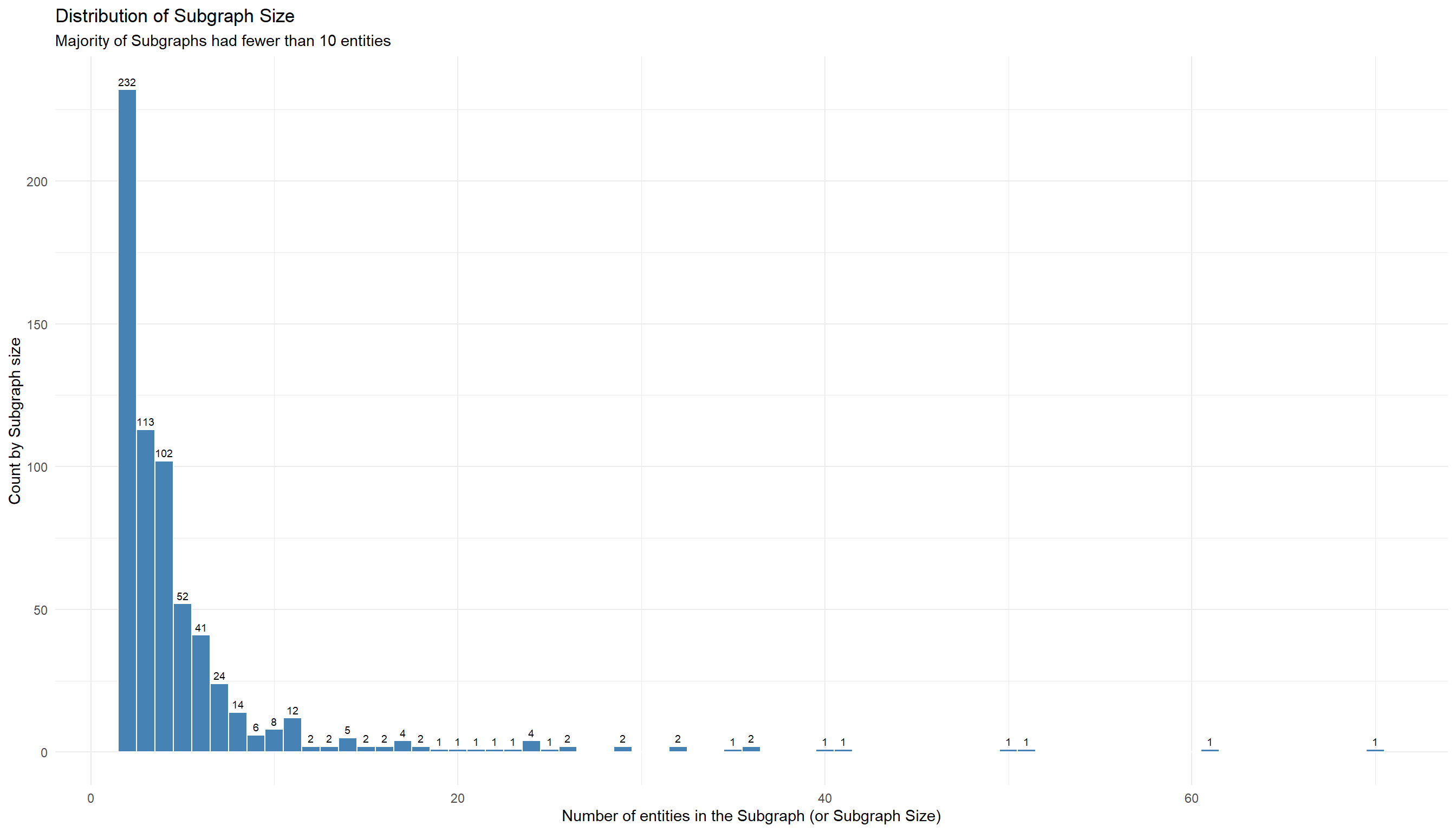

5. We computed the network diameter of the 648 business groups in the Seafood Network

To have a layered business structure within a subgraph, we will need the sub-graph’s network diameter to have a minimum value of 2 and above. The larger the diameter, the more complex the structure of the business group is.

Show the code

# get the list of group_ids for each subgraph in the network
subgraph_ids <- unique(freq_count$group_id)

# assign a diameter_list to store the results
diameter_list <- list()

# for each group_id
for (x in subgraph_ids) {
  
  # filter the relevant nodes for the group id
  nodes <- seafood_graph %>%
    activate(nodes) %>%
    as.tibble() %>%
    filter(group_id == x)
  
  # extract the relevant edge records   
  edges <- seafood_edges %>%
    filter(source %in% nodes$id| target %in% nodes$id)
  

  # construct the subgraph
  subgraph <- tbl_graph(nodes = nodes, 
                        edges = edges, 
                        directed = FALSE)
  
  # calculate the network diamter
  diameter <- with_graph(subgraph, graph_diameter())
  
  # append output to list
  diameter_list[[as.numeric(x)]] <- diameter
  
}

# 
network_diameter <- tibble(
  group_id = subgraph_ids,
  network_diameter = unlist(diameter_list)
)

6. We plotted the distribution of the network diameter of the 648 groups

Show the code

diameter <- network_diameter %>%
  count(network_diameter, sort = TRUE) %>%
  ggplot(aes(x = as.factor(network_diameter), y = n)) +
  geom_col(fill='#08519c') +
  xlab(NULL) +
  labs(x = "Network Diameter",
       y = "Count",
       title = "Distribution of Subgraphs by Network Diameter",
       subtitle = '4 Subgraphs had a diameterof 6 and above') +
  scale_x_discrete(breaks = 1:7) +
  geom_text(aes(label = n), vjust = -0.5) +
  theme_minimal() + 
  theme(axis.title.y = element_text(angle = 0, vjust = 0.5, hjust = 1))

diameter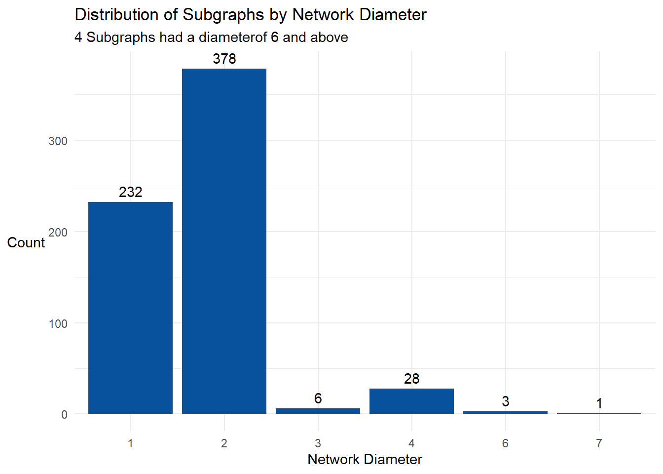

7. We combined the 2 sets of information obtained from Steps 5 and 6 on the subgraphs and displayed each group in a Jitterplot with Subgraph Size vs Network Diameter

Show the code

# Combine the subgraph size and the network_diamter into a single data frame
ratio <- freq_count %>%
  inner_join(network_diameter,by=c('group_id')) %>%
  mutate(size_to_diameter_ratio = round(count/network_diameter,2)) %>%
  arrange(desc(size_to_diameter_ratio))

# Display the information in a jitterplot
gg <- ggplot(ratio, 
            aes(x = network_diameter, 
                y = count,
                colour = network_diameter,
                tooltip = paste0('group id ',group_id,
                                 '<br> Group Size: ',count,
                                 '<br> Network Diameter: ',network_diameter),
                data_id = group_id)
            )+
  geom_jitter_interactive() +
  xlab("Network Diameter") +
  ylab("Subgraph Size") +
  ggtitle("Jitterplot of Subgraph Size vs Network Diameter") +
  theme_minimal() +
  scale_x_continuous(breaks = c(1,2,3,4,5,6,7)) +
  theme(legend.position = "none")
 
girafe(                                  
  ggobj = gg,                             
  width_svg = 6,                         
  height_svg = 6*0.618)

Observations:

• 2 subgraphs, at the extreme ends of the jitterplot, grabbed our attention:

  • Group ID 102: Short Network Diameter (2), High Subsgraph Size (61)

  • Group ID 210: Long Network Diameter (7), relatively High Subgraph Szie (40)

Before we proceeded to review the network diagram of these subgraphs, we created 3 functions to help us with our analysis:

(i) Function to extract the nodes and edges records of entities for a given subgraph.

Show the code

createNE_by_Group <- function(groupid) {

  
  relevant_entities <- seafood_graph %>%
    activate(nodes) %>%
    as.tibble()%>%
    arrange(id) %>%
    filter(group_id == groupid)


  relevant_edges <- mc3_edges_flat %>%
    filter(source %in% relevant_entities$id| target %in% relevant_entities$id) %>%
    rename(from = source) %>% 
    rename(to = target) %>% 
    mutate(title = type)

  # extract the seafood_nodes records using the edge information
  Cid1 <- relevant_edges %>%
    select(from) %>%
    rename(id = from)
  
  Cid2 <- relevant_edges %>%
    select(to) %>%
    rename(id = to)

  # Get unique nodes from source and target columns of edge records
  # left join with the mc3_nodes_cleaned3 dataset to get the attributes for the nodes
  relevant_nodes <- rbind(Cid1, Cid2) %>%
    distinct() %>%
    left_join(mc3_nodes_cleaned3,by=c('id')) %>%
    arrange(id) %>%
    mutate(label = id) %>%
    mutate(group = type) %>% 
    mutate(title = paste('id = ',id, "<br>Country =",country, '<br>Entity Type =',type,'<br>Revenue (omu) =',revenue_omu,'<br>Biz Category =',category,'<br>Biz Activity =',product_services))
  
  title = paste("Subsidiary Group ID",groupid)
  
  list(relevant_edges = relevant_edges, relevant_nodes = relevant_nodes, title = title)
   
}

(ii) Function to first identify the subgraph group id of a given entity and then extract the nodes and edges entity’s subgraph

This generates the nodes and edges data frames of a 2-hop network graph of the given entity which would facilitate our examination of the entity.

Show the code

createNE_by_id <- function(entityid) {
  
  # obtain the subgraph group id of the entity
  groupid <- seafood_graph %>% 
  activate(nodes) %>%
  filter(id == entityid) %>%
    select(group_id) %>%
    as.tibble()
  
  # assign the group id to a variable
  groupid <- groupid$group_id[1]
  
  # pass the group id into the createNE_by_Group() function to generate the subgraph
  output <- createNE_by_Group(groupid)
  
  # return the nodes and edges data frames for graphing
  list(relevant_edges = output$relevant_edges,relevant_nodes = output$relevant_nodes,title = entityid)
   
}

(ii) Function to plot an interactive Network graph with the given nodes and edges data

Show the code

createGraph <- function(r_nodes , r_edges,title) {
  visNetwork(nodes = r_nodes,   # Visualize the nodes
             edges = r_edges,   # Visualize the edges
             main = paste("Network graph of", title),
             height = "500px", width = "100%") %>%
    visIgraphLayout(layout = "layout_nicely") %>%
    visEdges(smooth = list(enables = TRUE, type = 'straightCross'),  # Customize the appearance of edges
             shadow = FALSE,
             dash = FALSE) %>%
    visGroups(groupname = "Company", shape = "icon", 
              icon = list(code = "f1ad", size = 75)) %>%  # Define a group with icon shape for companies
    visGroups(groupname = "Beneficial Owner", shape = "icon", 
              icon = list(code = "f007", color = "red")) %>%  # Define a group with red icon shape for beneficial owners
    visGroups(groupname = "Company Contacts", shape = "icon", 
              icon = list(code = "f007", color = "blue")) %>%  # Define a group with blue icon shape for company contacts
    visGroups(groupname = "Beneficial Owner, Company Contacts", shape = "icon", 
              icon = list(code = "f007", color = "purple")) %>%  # Define a group with purple icon shape for both beneficial owners and company contacts
    addFontAwesome() %>%  # Add Font Awesome icons to the visualization
    visOptions(highlightNearest = list(enabled = TRUE, degree = 1, hover = TRUE),  # Enable highlighting of nearest nodes on hover
               nodesIdSelection = TRUE,
               selectedBy = "group") %>%  # Enable node selection by group
    visInteraction(hideEdgesOnDrag = TRUE) %>%  # Hide edges while dragging nodes
    visLegend() %>%  # Display legend
    visLayout(randomSeed = 123)  # Set a random seed for consistent layout
}

3.1.1 Subgraph Group ID 102

First, we plotted the interactive network of Subgraph Group 102.

Show the code

result <- createNE_by_Group(102)
createGraph(result$relevant_nodes,result$relevant_edges, result$title) 

Network graph of Subsidiary Group ID 102

Select by idAlison PageAmanda SaundersAmanda ZimmermanAndrew FloresAngela RiggsAnthony FosterAnthony SotoArthur ThompsonAshley LyonsBahía de Plata SubmarineBrittney BondBrittney CrawfordCaracola del Mar A/SCarl HayesCarl NunezCarlos AlexanderCassie RobinsonCatherine AndersonChristie SimmonsChristine OrozcoCongo Rapids Ltd. CorporationCoral del Mar SE UnitedDaniel MartinezDavid DiazDeborah Torres DDSDebra ClineDonna BrownDonna WatsonElizabeth GonzalezGuzman, Fuller and HayesHeather MillerHeather PenningtonJanice WyattJason SuttonJay MitchellJennifer FlemingJeremy LeeJon HawkinsJoseph ObrienJulie StewartKimberly OconnorKrystal AndradeLuis GeorgeMatthew WheelerMegan BrownMichael HendersonMonique YoderNatasha DavisNiger Bend AS ExpressRobert Brown Jr.Robert StewartSandra MitchellSarah GonzalesSenegal Coast Ltd. Liability CoShannon AyalaStacy GrayStephanie BarnesStephanie BrooksSteve HortonSteven MurrayTabitha YuTheresa JacksonThomas PerezThomas SmithTimothy AbbottVictoria ChavezViento y Mar A/SWilliam Fisherjīng Coral LLC Carriers

---

Select by groupBeneficial OwnerBeneficial Owner, Company ContactsCompanyCompany Contacts

Congo had many BOs and we wondered if this was normal for companies in the edge data frame that was provided. As such, we derived the 95% Quantile Interval (QI) for number of BOs that companies had and noticed that 95% of the companies only had 1 to10 BOs.

Show the code

avg_BOs <- mc3_edges_flat %>%
  filter(type == 'Beneficial Owner') %>%
  group_by(source) %>%
  summarise(BO_count = n()) 
  
# Calculate the 95% quantile interval
lower_ci <- quantile(avg_BOs$BO_count, 0.025)
upper_ci <- quantile(avg_BOs$BO_count, 0.975)

# Create the histogram
ggplot(avg_BOs, aes(x = BO_count)) +
  geom_histogram(binwidth = 1, fill = "lightblue", color = "black") +
  labs(title = "Histogram of BO_count", x = "BO_count", y = "Frequency") +
  theme_minimal() +
  annotate("text", x = mean(avg_BOs$BO_count), y = 10,
           label = paste("95% QI:", lower_ci, "-", upper_ci), hjust = -0.1, vjust=-5, color = "red") +
  xlim(0, 40)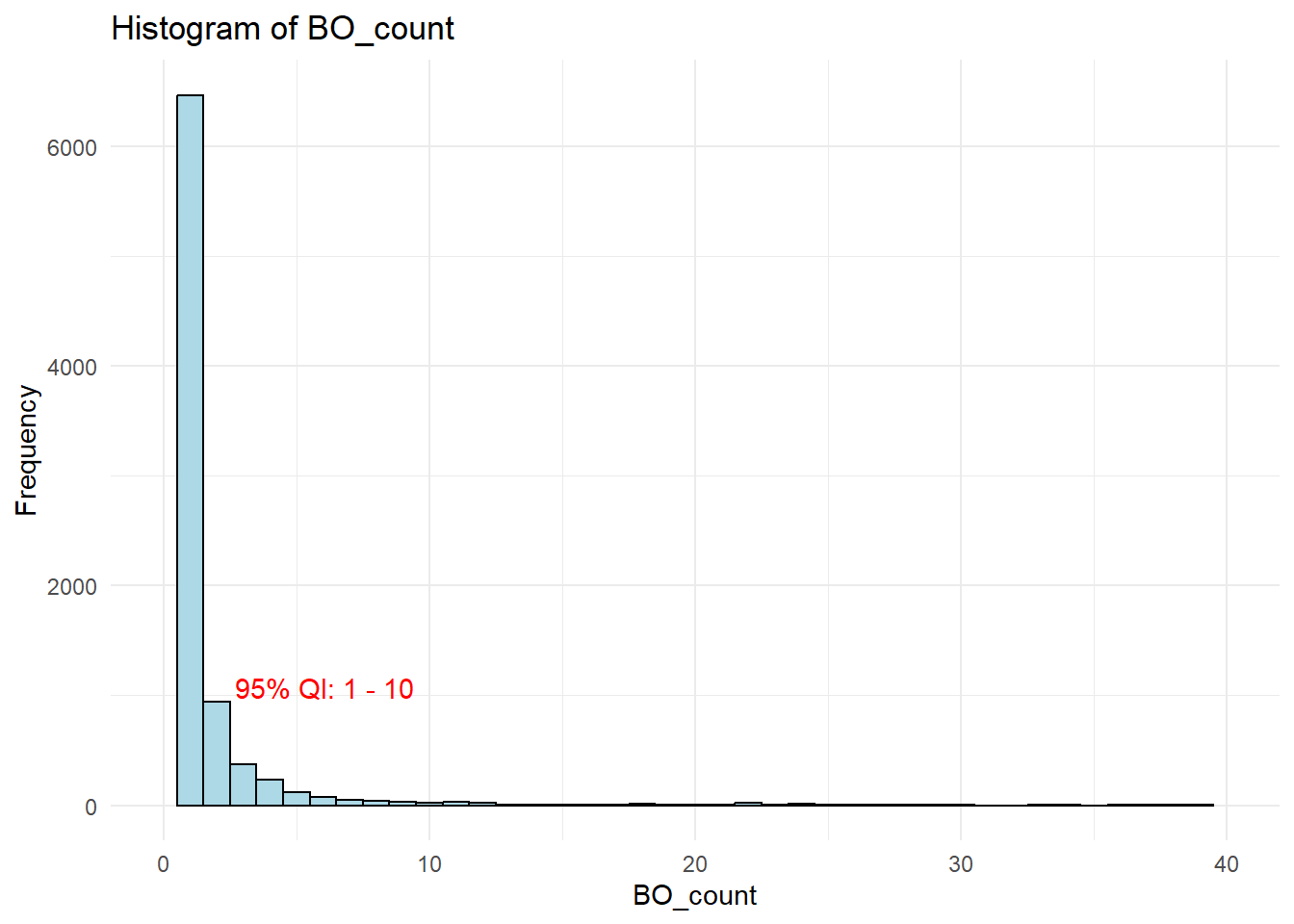

Anomaly 1: Multiple Beneficial Owners surrounding a Seafood Company, Congo Rapids Ltd. Corporation (Congo)

Cogno had 58 BOs, way beyond what a typical company had. One reasonable explanation, judging from the the range of products and services that Congo offered, could be that it was a large scale co-operation with many subsidiaries. However, it could also be a red-flag 🚩 for IUU as this would allow vessel owners to shop and select the vessel flag state of a BO that would facilitate their illicit activities, such as gaining access to fisheries resources which are reserved for vessels owned by a resident BO.

3.1.2 Subgraph Group ID 210

Similarly, we started our review with the network diagram of Subgraph Group 210.

Show the code

result <- createNE_by_Group(210)
createGraph(result$relevant_nodes,result$relevant_edges, result$title)

Network graph of Subsidiary Group ID 210

Select by idAlex BradleyAlexandria MarquezArunachal Pradesh s ОАОBrian LynchBrown PLCBrown, Noble and KruegerCarolyn PhillipsCharles MartinChristopher TerryCole NewtonCrosby, Davis and PatrickCurtis FullerDaniel SmithDanielle LopezDenise TurnerDesiree GonzalezHayley MullenHeather CastanedaJackson, Wilson and StarkJacob Fox IIIJames BerryJames GonzalezJennifer WilsonJennifer YoungJillian MooreJoseph MartinKeith PierceKenneth PerryKerala Market SRL WaveKim DavisKimberly WilliamsLaura MeyerMargaret GarciaMark DavisMediterranean s Worldwide UnderwaterMichael GonzalesMike LunaMr. Patrick MorrisonOliver-GrayPoole GroupRajasthan Market Limited Liability CompanyReef Rascals S.A. de C.V.Ricky SmithSaharan Coast Pic ForwadingSarah BurkeScottish Herring Lighthouse LLC SolutionsSeaScape Foods Ltd FreightShannon JensenTanya YoungThe Salted Pearl - Oyj Marine conservationTorres LtdTorres-HarveyTriton Seabass Sp ExportWest Bengal Ltd. Corporation Sandbarnián yú GmbH Investment

---

Select by groupBeneficial OwnerBeneficial Owner, Company ContactsCompanyCompany Contacts

Group ID 210 also shared the same observation as Group ID 102 of having multiple BOs for its seafood companies (Kerala Market SRL Wave and The Salted Pearl - Oyj Marine conservation), although the extent of having multiple BOs was not as serious as Congo’s. Both companies had 16 BOs.

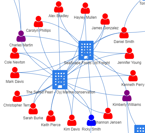
However, what struck us was the ownership structure of 2 entities in the network, The Salted Pearl - Oyj Marine conservation and SeaScape Foods Ltd Freight.

Anomaly 2: Multiple and Same Set of Individuals Associated with 2 Companies

In the image on the right below, we saw that The Salted Pearl - Oyj Marine Conservation and SeaScape Foods Ltd Freight sharing the same set of 16 BOs and 1 Company Contact. This appeared to be a deliberate arrangement to perpetuate a scheme 🚩 .

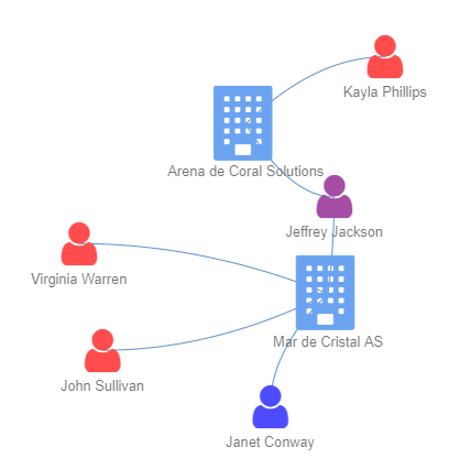
A more typical arrangement for 2 associated companies would be that they may share some common owners or contact persons, but not exactly the same set of individuals, similar to the setup for 2 seafood companies on the left image below.

Common: 2 companies may share some common owners or contact persons, but not exactly the same set of individuals	Uncommon: Multiple and Same Set of Individuals for 2 companies

3.2 Companies with “extraordinary” revenue

Companies exist to create profit for their owners. A larger company would generate more revenue and in our context, we used the number of BOs as a proxy for the company size. Let us check out the distribution of revenue generated per BO for each company in the Seafood Network.

Show the code

# find out the number of BOs (Company Contacts excluded) for every company
BO_for_company <- seafood_edges %>%
  filter(!type == 'Company Contacts') %>%
  group_by(source) %>%
  summarise(BO_count = n())

# compute revenue (in OMU) per BO per company
revenue_per_BO <- seafood_nodes %>%
  inner_join(BO_for_company, by=c("id"="source")) %>%
  # for this analysis, we will impute revenue_omu as 1 so that they can be considered in the analysis
  mutate(revenue_per_BO = ifelse(is.na(revenue_omu), 1,round(revenue_omu/BO_count,0)),
         # given the wide range of revenue, we applied log on the revenue_per_BO
         log_revenue = log(revenue_per_BO))

# Boxplot of the log_revenue of the Revenue per BO per company
p <- revenue_per_BO %>%
  ggplot(aes(x=type, y = log_revenue)) +
  geom_boxplot_interactive(
            aes(fill=category,
                group = paste(type,category),
                data_id = category,
                tooltip = after_stat({
                                      paste0(
                                        "Quartile (in Revenue_OMU):",
                                        "\nQ1: ", exp(.data$ymin),
                                        "\nQ3: ", exp(.data$ymax),
                                        "\nmedian: ", round(exp(.data$middle),0)
                                        )
                                      }),
                outlier.tooltip = paste("id:", id,
                                    "<br>Country:", country,
                                    "<br>Revenue:", revenue_omu,
                                    "<br>No. of BOs:", BO_count,
                                    "<br>Revenue Per BO:", revenue_per_BO,
                                    "<br>Biz Category:", category,
                                    "<br>Biz Acitivity:",product_services)
               ),
              outlier.colour='red') +
              theme(axis.title.x=element_blank(),
                  axis.text.x=element_blank(),
                  axis.ticks.x=element_blank()) +
              theme_minimal() + 
              coord_flip() +
  ggtitle("Boxplot of Revenue Per BO Per Seafood Company") +
  theme(axis.title.y = element_text(angle = 0, vjust = 0.5, hjust = 1))
          

girafe(                                  
  ggobj = p,                             
  width_svg = 6,                         
  height_svg = 6*0.618                      
)                                        

Mousing over the red outlier points on the right side of the plot, we have 3 entities with exceptionally high Revenue per BO. They were Baker and Sons, Barron LLC, Caracola del Mar NV Family. Let’s take a look at their networks.

3.2.1 Network Graph Comparison of Top 3 Entities with Highest Revenue Per BO

We plotted the network graph for Baker and Sons below and did the same for the other 2 entities.

Show the code

result<-createNE_by_id("Baker and Sons")
createGraph(result$relevant_nodes,result$relevant_edges,result$title)

Network graph of Baker and Sons

Select by idBaker and SonsChen, Jones and DavisCynthia PalmerFaroe Islands Ltd ExpressHancock IncJenna WilsonJones, Kennedy and JohnsonKnight-BrownMelissa AndersonMichael JohnsonMiller, Wiggins and SmithPerla del Mar Ges.m.b.H. MusselSeaBass Leska N.V. InternationalSeashell Seekers ОАО InternationalThompson LLC

---

Select by groupBeneficial OwnerBeneficial Owner, Company ContactsCompany

Anomaly 3: BO of a seafood company, Baker and Sons, having a number of other unrelated businesses

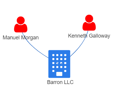
Other than owning another company (Faroe Islands Ltd Express) associated with seafood, we noticed one BO of Baker and Sons, Michael Johnson, owned a number of other companies that were unrelated to the seafood businesses. This structure was in contrast with the other 2 high revenue per BO entities, Barron LLC and Caracola del Mar NV Family as shown below, where the BOs only had 1 company to manage.

Barron LLC	Caracola del Mar NV Family

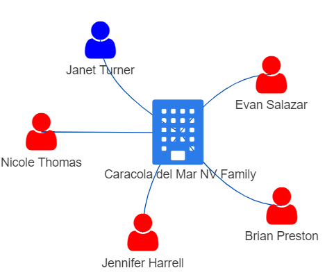While having a BO with numerous businesses unrelated to fishing does not directly imply involvement in illegal fishing, there’s a possibility that such unrelated business could be a front to launder illicit gains from IUU or act as a false front for other illegal activities 🚩. Fisheye could consider analysing the entity’s financial transactions, including sources of funding, payment flows,to look for any suspicious patterns, such as large amounts of cash transactions or frequent transfers to offshore jurisdictions known for illegal fishing activities.

3.2.2 Network Graph of Company with Low Revenue Per BO

Using the revenue per BO information that we generated earlier, we charted a scatter plot using Log Revenue Vs Number of BOs of Companies to identify companies with very low revenue per BO. Such entities would appear very close to the x-axis of the plot.

Show the code

plot_ly(data = revenue_per_BO %>%
          # Excluded the 3 entities with high revenue per BO to see the plot
          filter(log_revenue<=13.41), 
        x = ~BO_count, 
        y = ~revenue_omu,
        text = ~paste("Entity:", id,     
                      "<br>Country:", country,
                      "<br>Revenue:", revenue_omu,
                      "<br>No. of BOs:", BO_count,
                      "<br>Revenue Per BO:", revenue_per_BO,
                      "<br>Biz Category:", category),
                        
        color = ~revenue_per_BO, 
        colors = colorRampPalette(c("blue", "red"))(nrow(revenue_per_BO)))  %>%
      layout(title = 'Log Revenue vs No. Of BOs of Companies')

We would expect companies with lower revenue to be of smaller operating scale and had fewer BOs as seen from the clustered points at the point of origin in the scatter plot above. One such exception was Rufiji Delta GmbH Express (Rufiji).

Anomaly 4: Companies with little revenue and yet a substantial number of BOs.

Rufiji was an “exceptional” entity among the companies in the seafood sector, with a remarkably high number of BOs. It had 39 BOs while its revenue was only OMU 6137. This meant that each BO received an average of OMU 157, which was far below the median revenue per BO of OMU 12,429 for the sector (check out the boxplot above). The reasons for this unusual situation were not clear from the data.

Let’s check out the subgraph of Rufiji.

Show the code

result<-createNE_by_id("Rufiji Delta  GmbH Express")
createGraph(result$relevant_nodes,result$relevant_edges,result$title)

Network graph of Rufiji Delta GmbH Express

Select by idAlyssa DavisAndrew RamosAntonio LoweArena del Sol SaglBradley ThompsonChristopher Sanders DDSDanielle Conley PhDDawn SmithDonna BowmanEdward RichardErica AlexanderErin EdwardsGerald SandovalGreek Mackerel Cargo DredgeJason AndersonJeffrey MartinezJennifer VillanuevaKaren PhillipsKathleen MorrisKathryn AcevedoKatie CarrollMallory RobinsonMark GillMatthew MendozaMichael FullerMichael PattersonMichelle HudsonMolly PerryMorales, Herman and FletcherNeptune's Bounty SE GreenNicole MccarthyNolan-CrawfordOcéano del Este CoPatrick WhiteRichard HardyRufiji Delta GmbH ExpressSally LawrenceSally MillerSandra BeardSpencer CampbellStanley-GriffinStephen WellsSuzanne SaundersSydney BerryTina MarquezTrevor HernandezVictoria HallWilliam ChenWilliams, Mitchell and Taylor

---

Select by groupBeneficial OwnerBeneficial Owner, Company ContactsCompany

From the network, only 7 out of 39 BOs had an alternate source of income from another company. There was no other data that discloses how the rest of the BOs earned their living. This raised some questions about their economic situation and sustainability, and if there were commercially justifiable reasons for having a large pool of BOs 🚩 .

3.3 Business Groups with Presence in Multiple Countries

For each business group, we computed the number of countries in which the entities in the group had presence in. Thereafter, we constructed a jitterplot using Subgraph Size vs Number of Countries that the business groups operated in.

Show the code

# Combine the countries for each business group
country_count <- seafood_graph %>%
  activate(nodes) %>%
  as_tibble() %>%
  group_by(group_id) %>%
  summarise(country = paste(country, collapse = ", "),
            size = n()) %>%
  ungroup()

# Function to count unique words in a country column
unique_words <- function(text) {
  text_words <- str_split(text, ",\\s*")[[1]]
  text_words <- unique(text_words)
  text_words <- text_words[text_words != "NA"]
  unique_text_words <- unique(text_words)
  return(unique_text_words)
}

# Derive the unique contries and number of unique countries for each group
country_count <- country_count %>%
  mutate(unique_countries = map(country, unique_words)) %>%
  mutate(country_count = lengths(unique_countries))


# Display the information in a jitterplot
gg <- ggplot(country_count, 
            aes(x = country_count, 
                y = size,
                colour = country_count,
                tooltip = paste0('group id ',group_id,
                                 '<br> Group Size: ',size,
                                 '<br> Unique Countries Count: ',country_count,
                                  '<br> Unique Countries: ', unique_countries),
                data_id = group_id)
            )+
  geom_jitter_interactive() +
  xlab("No of Unique Countries that the Business Group Operated In") +
  ylab("Subgraph Size") +
  ggtitle("Jitterplot of Subgraph Size vs Countries of Operation") +
  theme_minimal() +
  scale_x_continuous(breaks = c(1,2,3,4,5,6,7,8,9,10)) +
  theme(legend.position = "none")
 
girafe(                                  
  ggobj = gg,                             
  width_svg = 6,                         
  height_svg = 6*0.618)

The obvious outlier in the plot was Subgraph Group ID 29, which operated in 10 countries.

3.3.1 Subgraph Group ID 29

The network graph for Subgraph Group ID 29 is as shown.

Show the code

result <- createNE_by_Group(29)
createGraph(result$relevant_nodes,result$relevant_edges, result$title)

Network graph of Subsidiary Group ID 29

Select by idAgua Ltd. Liability CoAnthony HunterAqua Aura SE Marine lifeBlueWater Bistro GmbH IndustrialBrewer IncCaracola del Este EnterprisesCasey Griffin Jr.Christopher StricklandCollins-PerezCoral del Mar SE UnitedCraig LeeCynthia MurphyDale RhodesDawn Morris MDDean-FisherDominguez, Marks and CollierDr. Danielle MaxwellDr. Lisa Gonzalez MDFrederick GreenHayley BrownHeather EricksonIrish Mackerel S.A. de C.V. Marine biologyJames CrossJames MartinezJennifer BauerJennifer DuarteJesus McclureJillian WhiteJohn HerreraJonathan HallKevin GarciaKristina DrakeLance WilsonLauren RobinsonLeah CruzLeon PittmanLimpopo River Ltd. Liability CoLisa McgrathLisa ValentineLtd. Corporation Ltd. CorporationMar de la Luz Oyster Sp HoldingsMark SimmonsMark TuckerMary RobinsonMichael BellMichael SotoMiss Gloria OwensMrs. Amy GravesNorwegian King Crab BVPeter ByrdPhillip BrewerPhyllis LanePunjab s Pic ExpressRachel SanfordRebecca SotoReynolds-DuncanSarah BarrettSeaside Summit Solutions EstuaryShannon SnyderStacy FloresStephanie MccallThomas SnyderTraci DavisTracy HarrisVanessa MccartyWilliam Solisshí rén yú Rybachit

---

Select by groupBeneficial OwnerBeneficial Owner, Company ContactsCompanyCompany Contacts

The main entity in subgraph was Aqua Aura SE Marine life (Aqua) which had presence in 9 countries. It not only operated in multiple countries, it also had a high number of beneficial owners (36 BOs) and contact persons (10 company contacts). There was no revenue information on Aqua even though one country which it traded in was Ocenanus.

Anomaly 5: Companies with presence in a high number of countries

Aqua was involved in wide range of business activities and hence, the large pool of individuals and high number of countries which it was associated with appeared legititmate. Nonetheless, business groups that operated in multiple countries and involving numerous individuals could create a complex and opaque structure, making it challenging to track and regulate the group’s fishing activities effectively. This structual complexity could be exploited to engage in illegal practices, such as evading regulations, concealing illegal fishing operations, or engaging in illicit activities along the seafood supply chain. As such, they could be of concern as well 🚩.

4.Conclusion

The lack of sufficient data hindered our ability to confirm our suspicion that some 🚩 illicit activities 🚩 were indeed taking place among the different business entities engaged in seafood commerce. However, our approach to detect anomalies using network attributes, revenue and country presence, would provide a good foundation for more in-depth investigation.

The exercise has been especially challenging, requiring a variety of data processing and manipulation techniques ranging from natural language processing to social network analysis. This is on top of the visual analytics skills that we have to apply to detect anomalies. On the positive side, it has exposed us to different aspects of data analytics and how they can be integrated to solve complex problems.

5.References

• Take-home Exercise 3: Kick-starter, Dr. Kam Tin Seong, Associate Professor of Information Systems (Practice), ISSS608 - Take-home Exercise 3 (isss608-ay2022-23apr.netlify.app)

• The exploitation of company structures by illegal fishing operators, Trygg Mat Tracking, https://www.tm-tracking.org/post/illegal-fishing-operators-exploit-company-structures-to-cover-up-illegal-operations

• Text Mining for Social and Behavioral Research Using R, Zhiyong Zhang, Text Mining for Social and Behavioral Research Using R (psychstat.org)

• Options for visNetwork, an R package for interactive network visualisation, Options (datastorm-open.github.io)